Spatial Dynamics of Human Populations: Some Basic Models
Robert A. Hanneman
(robert.hanneman@ucr.edu)
Department of Sociology
University of California, Riverside
2005
Single-Population Spatial Dynamics
Material and information quantities may move from one place to another over time. In this section, we develop the most basic models of movement. We will be concerned with the movement of two (very abstract and general) kinds of quantities: material and information. And, we will examine three basic approaches to looking at how these quantities move in space: neighborhoods, distances, and networks.
Where the quantities are "conserved" material quantities that can be located in only one place at a time, we will call their movement "migration." One type of material quantity is human population, and talking about the "migration" of population from place to place is everyday language. We can also think about the "migration" of populations of other species (including disease vectors), bulk and luxury goods, and money.
Where the quantities are not "conserved" (i.e. information), we will call their movement "diffusion." Information differs from material in that it may move to a new location without leaving it's origin -- if I tell you something, we now both know it. The information/material or non-conserved/conserved distinction doesn't always handle all of the subtle aspects of the different kinds of things that move from place to place. But it will work well enough for our basic needs.
There are several ways that the idea of "space" is translated into formal expressions so that we can build models of spatial dynamics. We will be concerned with three different translations.
Neighborhoods conceptualize space as physically adjacent areas. Things move by leaving one space, and re-locating to an adjacent space. Most cellular automata and agent-based models use the neighborhood approach. Since our models operate on a grid (or lattice), the whole space is one of overlapping neighborhoods of adjacent cells. Theories of movement specify whether a quantity moves or not; and, if it does, in what direction (and sometimes, how many squares).
Distances conceptualize space as nearness-closeness (adjacency is, if you will, a special case of distance). Each point or area in the grid is at a fixed distance from each other point or area on the grid. Theories of movement specify whether a quantity moves or not; and, if it does, how far. Distances are often used in mathematical models of spatial phenomena, because they have an easy and general form that can be used for specifying effects of friction, gravity, and the like on the amount of mass that moves from one location to another.
Networks conceptualize space as either adjacency or distance -- but do not map these concepts in physical coordinates. Physical locations in the grid may be "adjacent" or at a distance of one unit from any other location -- depending of some underlying pattern of connection. Consider, for an example, how transport by aircraft connects places. Many places simply do not have any connection to any others. Many other places that are physically far apart (e.g. Los Angeles and Hong Kong) are actually quite close when mapped on the air transport network.
page table of contentsIn the "neighborhood" approach, quantities migrate or diffuse from each location to all adjacent locations. On a grid there are two alternative definitions of "adjacent locations." The von Neuman neighborhood consists of the four squares to the North, South, East, and West of a square; the Moore neighborhood consists of the eight squares located NW, N, NE, W, E, SW, S, and SE of a square.
a. material/migration
Suppose that we had a 3 by 3 space, with population all population located, initially, in the NW corner (square 1,1). Let us suppose that the birth and death rates of this population are constant and equal. Let us also suppose that a constant percentage of the population out-migrates in each period of time.
Let's suppose that mobility follows von Neuman neighborhood rules. What will the result look like?
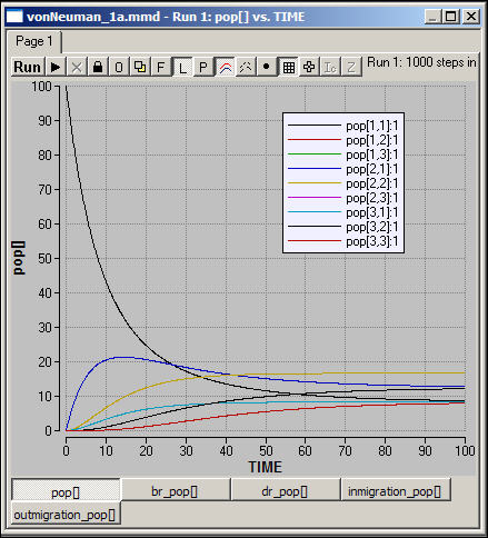
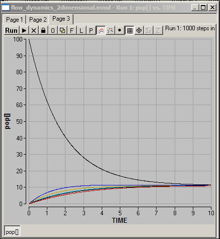
Figure 1a shows the levels of population in the nine squares as it changes over time.
Figure 1a. Stable population, constant migration across von Neuman neighborhoods.
Madonna program for figure 1a
Initial population data file for figure 1a
The level of population in the origin population declines exponentially until it converges with the levels of population in other corner squares. The squares immediately adjacent to the origin (1,2 and 2,1) rise rapidly before declining to the same equilibrium values as other "edge" squares (e.g. 2,3). The center square rises more rapidly than others (except those close to the point of origin), and is the largest population at equilibrium. Can you explain:
Alternatively, let's assume that migration followed Moore neighborhood rules. What will the result look like? Ask yourself:
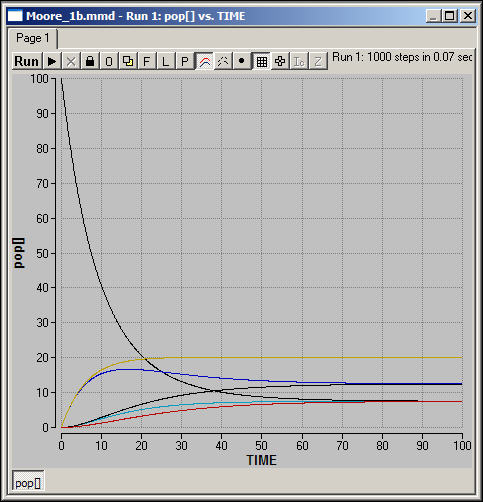
Figure 1b shows the same scenario as figure 1, but using Moore neighborhoods. Were you right?
Figure 1b. Stable population, constant migration across Moore neighborhoods.
Madonna program for figure 1b
Initial population data file for figure 1b
Things to try:
b. information/diffusion
If a quantity does not actually change location, but rather is "reproduced" or cloned to a new location when it diffuses, the overall dynamics of the system will look quite different.
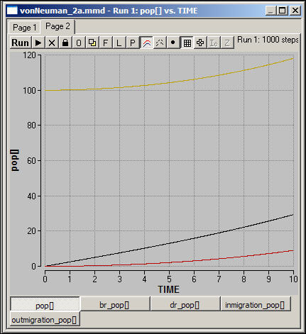
Figure 2a shows the dynamics of the diffusion of a conserved quantity over the first ten time periods. The information here (100 units) is initially located in the center of the grid (2,2). The diffusion here occurs across a von Neuman neighborhood.
Figure 2a. Information diffusion across von Neuman neighborhoods
Madonna program for figure 2a
Initial population data file for figure
Where your predictions correct?
One key difference is that the quantities in all locations grow exponentially, and the system does not have an equilibrium. This is because information is continuously cloned from all locations to it's neighbors, without being used up -- so it accumulates. Since the amount of information migrating is a constant proportion of the level of information in each population, the amount migrating continuously increases as the amount present in each location grows.
Notice that location does matter. The original point source of information always contains the largest amount, and the gap between it and it's neighbors widens over time. Squares that are further away from the starting point begin their growth later, and never catch up.
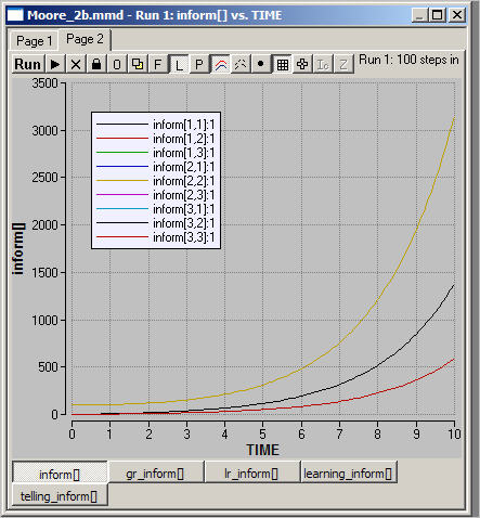
This type of conserved diffusion can also be mapped across Moore space. A simulation of this is shown as figure 2b.
Figure 2b. Information diffusion across Moore neighborhoods
Madonna program for figure 2b
Initial inform values for figure 2b
In this run, we have begun with information in the center of the grid.
The movements of some things may be efficiently modeled as functions of the physical distance between their locations on the grid. The attractiveness of a city as a destination for migration, for example, has been theorized to be an inverse function of the of it's distance from other places. Material may migrate from a place to all other places as a function of its distance from those places; information may diffuse with an intensity inversely proportional to physical distance.
There are a number of different ways of indexing the distance between two places in a grid. We will use the simple "Euclidean distance." The Euclidean distance between two points is equal to the square root of the sum of the differences in their X coordinates squared and their Y coordinates squared.
a. material/migration
Let's suppose, again, that we have a population located in the NW corner (cell 1,1) of a three-by-three grid. In each period of time, some proportion of this population migrates out. The destinations of these migrants are inversely proportional to the square of the distance from the origin. For example, migrants from (1,1) to (1,2; 2,2; and 2,1) are at a distance of 1, so migration is most intense to each of these locations. At the same time, however, migration occurs to (1,3 and 3,1), a distance of 2, with the intensity 1/2. The same is true for all the amount of migration from 1,1 to all other coordinates.
Once population reaches a new location, migration also begins from that location to all others, following the same rule of proportionality inverse to distance of the new location to all others.
Figure 3a shows a basic migration governed by the inverse distance rule, beginning in the NW corner.
Figure 3a. Migration with rates inversely proportional to distance
b. information/diffusion
The dynamics of information diffusion from a single point source to other locations can be specified in the same way (with flows of information from each location to all others being inversely proportional to distance). Since information does not actually "move," but rather is "copied to" other locations, the characteristic patterns differ greatly, as we see in figure 3b.
Figure 3b. Diffusion of information at rates inversely proportional to the square of distance from an initial single source
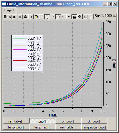
Since information is not "used up" by being shared, and since every location sends information to every other location, growth at all locations is exponential. Although the "message" started in the upper left corner (1,1), it is the central location (2,2) that soon comes to have the greatest accumulation. Can you see why central locations would have this advantage? (answer: because the central location has the smallest sum of distances from all other locations).
page table of contentsThe "space" or "distance" between social actors -- as they perceive it -- is often very different from the physical space between them. Actors may maintain close social ties over long physical distances; they may have very weak or no connection to actors who are physically close to them.
The distances between physical spaces, too, may not always resemble adjacency (as in neighborhoods) or physical distance (as in Euclidean distances). New York and Los Angeles are quite distant if I am traveling on foot, or even in an automobile; but they are quite close by air travel. To describe the distance from one place to another by air, the number of intermediate steps, rather than the physical distance may be more important.
A common way of representing connections among places (or social actors) that does not rely on physical space is to "map" them as locations in a network of connections. Consider the network (or "graph") in figure 4.
Figure 4. Simple modified "small world" network
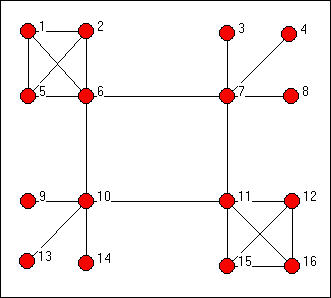
Imagine that locations 6, 7, 10, and 11 are seaports among which ships can travel (but that ships from each port travel directly only to the two ports adjacent to them. Locations 1, 2, and 5 are connected in a dense road network with the port (6). An analogous "country" consists of locations 11, 12, 15, and 16. In the two other "countries" (i.e. 7, 3, 4, 8; 10, 9, 13, 14) the port city is a central place, and all travel from one place to another in the country passes through it.
This particular network, while highly simplified, is not too atypical of many real-world "small -world" networks in which all actors have more ties to their local group or cluster than to outsiders (i.e. the graph is pretty highly clustered), but the average distance between any two points (even in distant countries) is quite small. For example, a person migrating from location 13 could reach location 4 in four steps. Most actors interact most of the time with others in their group (and the majority of actors have no connections at all outside their group); but, at the same time, a material or informational quantity can from from any actor to any other in the whole population with only a few intermediate stops.
a. material/migration
The network in figure 4 might provide a good way of describing migration flows. Migrations don't go from everywhere to everywhere -- they tend to much heavier along some pathways than others. And, most migration is "stepwise." First people move from the "village" (e.g. location 1) to the "city" (e.g. location 6), and then they may move to another city at great distance.
Let's imagine that we have a total population of 40 people. Ten each are located in the four "corners" of the network (i.e. 1, 4, 13, 16). Let's suppose that birth and death rates are in equilibrium (2% per year each) in all populations. Let's suppose that 10% of the population of any location moves each year, and that when it moves, it moves equally along each available network pathway. These are all very much over-simple assumptions, of course -- but they give us a starting point for understanding the effects of space itself on the outcome.
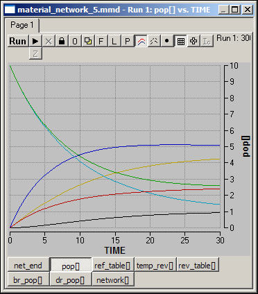
Figure 5 shows the curves that describe how the populations of the locations will change over time in this simple simulation.
Figure 5. Migration flow in a modified "small world" network
Madonna program for figure 5
Network structure for figure 5
Initial population values for figure 5
We can see that the populations of the four origin locations decline until they reach two different equilibrium levels (one for the two "cliques" and one for the two "star" communities in the graph). Central locations end up with higher populations at equilibrium than do peripheral locations; the blue and yellow curves describe the outcomes for the central locations. The total population in the two "clique" portions of the graph end up higher than in the stars. The distribution of final population is also more equal in cliques than in stars, and the central point of the stars has higher final values than the central points of the stars.
The equilibrium outcome is:
| 2.7 | 2.7 | 0.9 | 0.9 |
| 2.7 | 4.5 | 4.6 | 0.9 |
| 0.9 | 4.6 | 4.5 | 2.7 |
| 0.9 | 0.9 | 2.7 | 2.7 |
There are some interesting patterns here.
Ask yourself:
b. information/diffusion
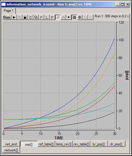
What if the quantity that was moving on a network-mapped space was non-conserved? That is, if it was replicated to the next network location, rather than migrating? Figure 6 shows the same experiment as figure 5, but this time the quantities are replicated along the network, rather than migrating.
Figure 6. Diffusion of information across the modified "small-world" network
Madonna program for figure 6
Network structure for figure 6
Initial populations for figure 6
Since information accumulates and propagates over the network, the level grows exponentially at all locations. The rates of growth, however, are not all equal. In fact, the same underlying patterns emerge as a result of the structure of the network: peripheral locations grow more slowly than central locations. Growth in tightly connected local neighborhoods is more rapid than growth in less tightly coupled neighborhoods. Rates of growth of centers of "stars" are higher than rates of growth of "cliques." The differences between the rate of growth in the core and in the periphery is greater in centralized "star" neighborhoods than it is in "clique" neighborhoods.
page table of contentsThe purpose of this chapter has been to introduce three ways of thinking about "space" and "distance" that are often useful in building models of social spatial dynamics. The ideas of "neighborhoods," "distances," and "networks" are three ways of representing the locations of social objects. Different approaches are more useful for different kinds of problems.
Neighborhood representations of space are commonly often used in agent-based-modeling and cellular automata. In neighborhood space, each actor is embedded in a set of adjacent actors, and the neighborhoods overlap to form a lattice. When material or information migrates or diffuses, it does so by moving from a neighborhood to adjacent neighborhoods. When actors "act" they often monitor or take into account the actions of their neighbors. We examined the two most common kinds of neighborhoods -- the von Neuman and Moore definitions. You might think about other definitions of neighborhoods that might apply to systems that interest you.
Distance representations of spatial relations (we looked at the most common approach -- Euclidean distance) are often useful when actors interact with, or share information with all other actors -- not just neighbors. Usually, the amount of migration or diffusion between "places" or "actors" in Euclidean space is some function of the distance between them. We explored migration and diffusion dynamics as a function of the inverse of the square of the distance between places or populations. You might think about other "functions" of distance that might apply to systems that interest you.
We also took a look at network representations of distance. Networks are maybe the most flexible approach to thinking about distance for many social science problems. von Neuman and Moore neighborhoods can also be represented as networks. Network conceptions of distance can have some properties that are quite interesting and useful for representing social relations. The distance from A to B does not have to be the same as the distance from B to A. Neighborhoods do not have to be homogeneous -- some actors can have large neighborhoods, and others small. The distances represented by networks can be "social" distances rather than physical distances. Actors may be connected in multiple ways by different networks, simultaneously (the movement of bulk material goods may follow one topology, the movement of persons may follow another).
Now that we have some of the basic ideas about spatial dynamics in hand, we can begin to build some models that are just a bit more realistic.