9. Ego networks
In the previous chapter we looked at the idea of the amount of "embedding" in whole networks -- loosely: the extent to which actors find themselves in social structures characterized by dense, reciprocal, transitive, strong ties. The main theme was to understand and index the extent and nature of the pattern of "constraint" on actors that results from the way that they are connected to others. These approaches may tell us some interesting things about the entire population and its sub-populations; but, they don't tell us very much about the opportunities and constraints facing individuals.
If we want to understand variation in the behavior of individuals, we need to take a closer look at their local circumstances. Describing and indexing the variation across individuals in the way they are embedded in "local" social structures is the goal of the analysis of ego networks.
We need some definitions.
"Ego" is an individual "focal" node. A network has as many egos as it has nodes. Egos can be persons, groups, organizations, or whole societies.
"Neighborhood" is the collection of ego and all nodes to whom ego has a connection at some path length. In social network analysis, the "neighborhood" is almost always one-step; that is, it includes only ego and actors that are directly adjacent. The neighborhood also includes all of the ties among all of the actors to whom ego has a direct connection. The boundaries of ego networks are defined in terms of neighborhoods.
"N-step neighborhood" expands the definition of the size of ego's neighborhood by including all nodes to whom ego has a connection at a path length of N, and all the connections among all of these actors. Neighborhoods of greater path length than 1 (i.e. egos adjacent nodes) are rarely used in social network analysis. When we use the term neighborhood here, we mean the one-step neighborhood.
"In" and "Out" and other kinds of neighborhoods. Most of the analysis of ego networks uses simple graphs (i.e. graphs that are symmetric, and show only connection/not, not direction). If we are working with a directed graph, it is possible to define different kinds of ego-neighborhoods. An "out" neighborhood would include all the actors to whom ties are directed from ego. An "in" neighborhood would include all the actors who sent ties directly to ego. We might want to define a neighborhood of only those actors to whom ego had reciprocated ties. There isn't a single "right" way to define an ego neighborhood for every research question.
"Strong and weak tie neighborhoods." Most analysis of ego networks uses binary data -- two actors are connected or they aren't, and this defines the ego neighborhood. But if we have measured the strength of the relation between two actors, and even its valence (positive or negative), we need to make choices about when we are going to decide that another actor is ego's neighbor. With ties that are measured as strengths or probabilities, a reasonable approach is to define a cut-off value (or, better, explore several reasonable alternatives). Where the information about ties includes information about positive/negative, the most common approach is to analyze the positive tie neighborhood and the negative tie neighborhood separately.
table of contentsEgo network data commonly arise in two ways:
Surveys may be used to collect information on ego networks. We can ask each research subject to identify all of the actors to whom they have a connection, and to report to us (as an informant) what the ties are among these other actors. Alternatively, we could use a two-stage snowball method; first ask ego to identify others to whom ego has a tie, then ask each of those identified about their ties to each of the others identified.
Data collected in this way cannot directly inform us about the overall embeddedness of the networks in a population, but it can give us information on the prevalence of various kinds of ego networks in even very large populations. When data are collected this way, we essentially have a data structure that is composed of a collection of networks. As the actors in each network are likely to be different people, the networks need to be treated as separate actor-by-actor matrices stored as different data sets (i.e. it isn't a good idea to "stack" the multiple networks in the same data file, because the multiple matrices do not represent multiple relations among the same set of actors).
A modification of the survey method can give rise to a multi-plex data structure (that is, a "stack" of actor-by-actor matrices of equal dimension). If we ask each ego to characterize their relation with the occupants of social roles (or a particular occupant of a role), and to also report on the relations among occupants of those roles, we can build "conformable" matrices for each ego. For example, suppose that we asked a number of egos: "do you have a male friend or friends in your classroom?" "Do you have a female friend or friends in your classroom?" and "Are your male friends, friends of your female friends?" The resulting data for each ego would have three nodes (ego, "male friends," "female friends") and the ties among them. Since each ego's matrix would have the same nodes (in the sense of social roles, but not individuals) they could be treated as a type of multi-plex data that we will discuss more later on.
The second major way in which ego network data arise is by "extracting" them from regular complete network data. The Data>Extract approach can be used to select a single actor and their ties, but would not include the ties among the "alters." The Data>Subgraphs from partitions approach could be used if we had previously identified the members of a particular ego neighborhood, and stored this as an attribute vector.
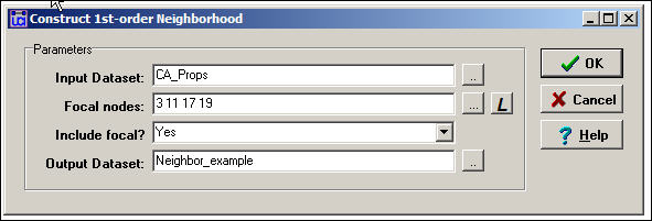
More commonly, though, we would want to extract multiple, or even all of the ego networks from a full network to be stored as separate files. For this task, the Data>Egonet tool is ideal. Here is an example of the dialog for using the tool:
Figure 9.1. Dialog for Data>Egonet
Here we are focusing on ballot proposition campaigns in California that are connected by having donors in common (i.e. CA_Props is a proposition-by-proposition valued matrix). We've said that we want to extract a network that includes the 3rd, 11th, 17th, and 19th rows/columns, and all the nodes that are connected to any of these actors. More commonly, we might select a single "ego." The list of focal nodes can be provided either as an attribute file, by typing in the list of row numbers, or by selecting the node labels of the desired actors.
A picture of part of the resulting data, stored as a new file called "Neighbor_example" is shown in figure 9.2.
Figure 9.2. (Partial) output of Data>Egonet
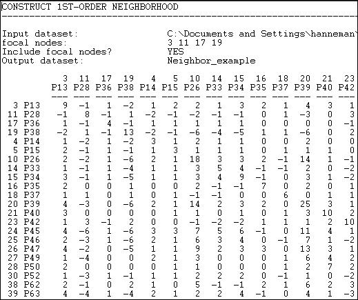
Extracting sub-graphs, based on a focal actor or set of actors (e.g. "elites") can be a very useful way of looking at a part of a whole network, or the condition of an individual actor. The Data>Egonet tool is helpful for creating data sets that are good for graphing and separate analysis -- particularly when the networks in which the focal actor/actors are embedded are quite large.
It is not necessary, however, to create separate ego-network datasets for each actor to be analyzed. The approaches to analysis that we'll review below generate output for the first-order ego network of every node in a dataset. For small datasets, there is often no need to extract separate ego networks.
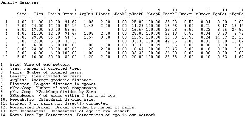
table of contentsThere are quite a few characteristics of the ego-neighborhoods of actors that may be of interest. The Network>Ego networks>Density tools in UCINET calculate a substantial number of indexes that describe aspects of the neighborhood of each ego in a data set. Here is an example of the dialog, applied to the Knoke information exchange data (these are binary, directed connections).
Figure 9.3. Dialog for Network>Ego networks>Density

In this example, we've decided to examine "out neighborhoods" (in neighborhoods or undirected neighborhoods can also be selected). We've elected not to save the output as a dataset (if you wanted to do further analysis, or treat ego network descriptive statistics as node attributes, you might want to save the results as a file for use in other routines or Netdraw). Here are the results:
Figure 9.4 Ego network density output for Knoke information out-neighborhoods
There's a lot of information here, and we should make a few comments.
Note that there is a line of data for each of the 10 organizations in the data set. Each line describes the one-step ego neighborhood of a particular actor. Of course, many of the actors are members of many of the neighborhoods -- so each actor may be involved in many lines of data.
Size of ego network is the number of nodes that one-step out neighbors of ego, plus ego itself. Actor 5 has the largest ego network, actors 6, 7, and 9 have the smallest networks.
Number of directed ties is the number of connections among all the nodes in the ego network. Among the four actors in ego 1's network, there are 11 ties.
Number of ordered pairs is the number of possible directed ties in each ego network. In node 1's network there are four actors, so there are 4*3 possible directed ties.
Density is, as the output says, the number of ties divided by the number of pairs. That is, what percentage of all possible ties in each ego network are actually present? Note that actor 7 and 9 live in neighborhoods where all actors send information to all other actors; they are embedded in very dense local structures. The welfare rights organization (node 6) lives in a small world where the members are not tightly connected. This kind of difference in the constraints and opportunities facing actors in their local neighborhoods may be very consequential.
Average geodesic distance is the mean of the shortest path lengths among all connected pairs in the ego network. Where everyone is directly connected to everyone (e.g. node 7 and 9) this distance is one. In our example, the largest average path length for connected neighbors is for actor 5 (average distances among members of the neighborhood is 1.57).
Diameter of an ego network is the length of the longest path between connected actors (just as it is for any network). The idea of a network diameter, is to index the span or extensiveness of the network -- how far apart are the two furthest actors. In the current example, they are not very far apart in the ego networks of most actors.
In addition to these fairly basic and reasonably straight-forward measures, the output provides some more exotic measures that get at some quite interesting ideas about ego neighborhoods that have been developed by a number of social network researchers.
Number of weak components. A weak component is the largest number of actors who are connected, disregarding the direction of the ties (a strong component pays attention to the direction of the ties for directed data). If ego was connected to A and B (who are connected to one another), and ego is connected to C and D (who are connected to one another), but A and B are not connected in any way to C and D (except by way of everyone being connected to ego) then there would be two "weak components" in ego's neighborhood. In our example, there are no such cases -- each ego is embedded in a single component neighborhood. That is, there are no cases where ego is the only connection between otherwise dis-joint sets of actors.
Number of weak components divided by size. The likelihood that there would be more than one weak components in ego's neighborhood would be a function of neighborhood size if connections were random. So, to get a sense of whether ego's role in connecting components is "unexpected" given the size of their network, it is useful to normalize the count of components by size. In our example, since there are no cases of multiple components, this is a pretty meaningless exercise.
Two-step reach goes beyond ego's one-step neighborhood to report the percentage of all actors in the whole network that are within two directed steps of ego. In our example, only node 7 cannot get a message to all other actors within "friend-of-a-friend" distance.
Reach efficiency (two-step reach divided by size) norms the two-step reach by dividing it by size. The idea here is: how much (non-redundant) secondary contact to I get for each unit of primary contact? If reach efficiency is high, then I am getting a lot of "bang for my buck" in reaching a wider network for each unit of effort invested in maintaining a primary contact. If my neighbors, on the average, have few contacts that I don't have, I have low efficiency.
Brokerage (number of pairs not directly connected). The idea of brokerage (more on this, below) is that ego is the "go-between" for pairs of other actors. In an ego network, ego is connected to every other actor (by definition). If these others are not connected directly to one another, ego may be a "broker" ego falls on a the paths between the others. One item of interest is simply how much potential for brokerage there is for each actor (how many times pairs of neighbors in ego's network are not directly connected). In our example, actor number 5, who is connected to almost everyone, is in a position to broker many connections.
Normalized brokerage (brokerage divided by number of pairs) assesses the extent to which ego's role is that of broker. One can be in a brokering position a number of times, but this is a small percentage of the total possible connections in a network (e.g. the network is large). Given the large size of actor 5's network, the relative frequency with which actor 5 plays the broker role is not so exceptional.
Betweenness is an aspect of the larger concept of "centrality." A later chapter provides a more in-depth treatment of the concept and its application to whole networks. For the moment, though, it' pretty easy to get the basic idea. Ego is "between" two other actors if ego lies on the shortest directed path from one to the other. The ego betweenness measure indexes the percentage of all geodesic paths from neighbor to neighbor that pass through ego.
Normalized Betweenness compares the actual betweenness of ego to the maximum possible betweenness in neighborhood of the size and connectivity of ego's. The "maximum" value for betweenness would be achieved where ego is the center of a "star" network; that is, no neighbors communicate directly with one another, and all directed communications between pairs of neighbors go through ego.
The ideas of "brokerage" and "betweenness" are slightly
differing ways of indexing just how "central" or "powerful"
ego is within their own neighborhood. This aspect of how an actor's
embedding may provide them with strategic advantage has received a great deal of
attention. The next two sections, on "structural holes" and
"brokerage" elaborate on ways of looking at positional opportunity and
constraint of individual actors.
table of contents
In several important works, Ronald Burt coined and popularized the term "structural holes" to refer to some very important aspects of positional advantage/disadvantage of individuals that result from how they are embedded in neighborhoods. Burt's formalization of these ideas, and his development of a number of measures (including the computer program Structure, that provides these measures and other tools) has facilitated a great deal of further thinking about how and why the ways that an actor is connected affect their constraints and opportunities, and hence their behavior.
The basic idea is simple, as good ideas often are.
Imagine a network of three actors (A, B, and C), in which each is connected to each of the others as in figure 9.5.
Figure 9.5. Three actor network with no structural holes

Let's focus on actor A (of course, in this case, the situations of B and C are identical in this particular network). Suppose that actor A wanted to influence or exchange with another actor. Assume that both B and C may have some interest in interacting or exchanging, as well. Actor A will not be in a strong bargaining position in this network, because both of A's potential exchange partners (B and C) have alternatives to treating with A; they could isolate A, and exchange with one another.
Now imagine that we open a "structural hole" between actors B and C, as in figure 9.6. That is, a relation or tie is "absent" such that B and C cannot exchange (perhaps they are not aware of one another, or there are very high transaction costs involved in forming a tie).
Figure 9.6. Three actor network with a structural hole

In this situation, actor A has an advantaged position as a direct result of the "structural hole" between actors B and C. Actor A has two alternative exchange partners; actors B and C have only one choice, if they choose to (or must) enter into an exchange.
Real networks, of course, usually have more actors. But, as networks grow in size, they tend to become less dense (how many relations can each actor support?). As density decreases, more "structural holes" are likely to open in the "social fabric." These holes, and how and where they are distributed can be a source of inequality (in both the strict mathematical sense and the sociological sense) among actors embedded in networks.
Network>Ego Networks>Structural Holes examines the position of each actor in their neighborhood for the presence of structural holes. A number of measures (most proposed by Burt) that describe various aspects of the advantage or disadvantage of the actor are also computed. Figure 9.7 shows a typical dialog box; we're looking at the Knoke information network again.
Figure 9.7. Network>Ego Networks>Structural Holes dialog

Measures related to structural holes can be computed on both valued and binary data. The normal practice in sociological research has been to use binary (a relation is present or not). Interpretation of the measures becomes quite difficult with valued data (at least I find it difficult). As an alternative to losing the information that valued data may provide, the input data could be dichotomized (Transform>Dichotomize) at various levels of strength. The structural holes measures may be computed for either directed or undirected data -- and the interpretation, of course, depends on which is used. Here, we've used the directed binary data. Three output arrays are produced, and can be saved as separate files (or not, as the output reports all three).
The results are shown in figure 9.8, and need a bit of explanation.
Figure 9.8. Structural holes results for the Knoke information exchange network

Dyadic redundancy means that ego's tie to alter is "redundant." If A is tied to both B and C, and B is tied to C (as in figure 9.5) A's tie to B is redundant, because A can influence B by way of C. The dyadic redundancy measure calculates, for each actor in ego's neighborhood, how many of the other actors in the neighborhood are also tied to the other. The larger the proportion of others in the neighborhood who are tied to a given "alter," the more "redundant" is ego's direct tie. In the example, we see that actor 1's (COUN) tie to actor 2 (COMM) is largely redundant, as 72% of ego's other neighbors also have ties with COMM. Actors that display high dyadic redundancy are actors who are embedded in local neighborhoods where there are few structural holes.
Dyadic constraint is an measure that indexes the extent to which the relationship between ego and each of the alters in ego's neighborhood "constrains" ego. A full description is given in Burt's 1992 monograph, and the construction of the measure is somewhat complex. At the core though, A is constrained by its relationship with B to the extent that A does not have many alternatives (has few other ties except that to B), and A's other alternatives are also tied to B. If A has few alternatives to exchanging with B, and if those alternative exchange partners are also tied to B, then B is likely to constrain A's behavior. In our example constraint measures are not very large, as most actors have several ties. COMM and MAYR are, however, exerting constraint over a number of others, and are not very constrained by them. This situation arises because COMM and MAYR have considerable numbers of ties, and many of the actors to whom they are tied do not have many independent sources of information.
Effective size of the network (EffSize) is the number of alters that ego has, minus the average number of ties that each alter has to other alters. Suppose that A has ties to three other actors. Suppose that none of these three has ties to any of the others. The effective size of ego's network is three. Alternatively, suppose that A has ties to three others, and that all of the others are tied to one another. A's network size is three, but the ties are "redundant" because A can reach all three neighbors by reaching any one of them. The average degree of the others in this case is 2 (each alter is tied to two other alters). So, the effective size of the network is its actual size (3), reduced by its redundancy (2), to yield an efficient size of 1.
Efficiency (Efficie) norms the effective size of ego's network by its actual size. That is, what proportion of ego's ties to its neighborhood are "non-redundant." The effective size of ego's network may tell us something about ego's total impact; efficiency tells us how much impact ego is getting for each unit invested in using ties. An actor can be effective without being efficient; and and actor can be efficient without being effective.
Constraint (Constra) is a summary measure that taps the extent to which ego's connections are to others who are connected to one another. If ego's potential trading partners all have one another as potential trading partners, ego is highly constrained. If ego's partners do not have other alternatives in the neighborhood, they cannot constrain ego's behavior. The logic is pretty simple, but the measure itself is not. It would be good to take a look at Burt's 1992 Structural Holes. The idea of constraint is an important one because it points out that actors who have many ties to others may actually lose freedom of action rather than gain it -- depending on the relationships among the other actors.
Hierarchy (Hierarc) is another quite complex measure that describes the
nature of the constraint on ego. If the total constraint on ego is
concentrated in a single other actor, the hierarchy measure will have a higher
value. If the constraint results more equally from multiple actors in
ego's neighborhood, hierarchy will be less. The hierarchy measure, in
itself, does not assess the degree of constraint. But, among whatever
constraint there is on ego, it measures the important property of dependency --
inequality in the distribution of constraints on ego across the alters in its
neighborhood.
table of contents
Burt's approach to understanding how the way that an actor is embedded in its neighborhood is very useful in understanding power, influence, and dependency effects. We'll examine some similar ideas in the chapter on centrality. Burt's underlying approach is that of the rational individual actor who may be attempting to maximize profit or advantage by modifying the way in which they are embedded. The perspective is decidedly "neo-classical."
Fernandez and Gould also examined the ways in which actor's embedding might constrain their behavior. These authors though, took a quite different approach; they focus on the roles that ego plays in connecting groups. That is, Fernandez and Gould's "brokerage" notions examine ego's relations with its neighborhood from the perspective of ego acting as an agent in relations among groups (though, as a practical matter, the groups in brokerage analysis can be individuals).
To examine the brokerage roles played by a given actor, we find every instance where that actor lies on the directed path between two others. So, each actor may have many opportunities to act as a "broker." For each one of the instances where ego is a "broker," we examine which kinds of actors are involved. That is, what are the group memberships of each of the three actors? There are five possible combinations.
In figure 9.9, the ego who is "brokering" (node B), and both the source and destination nodes (A and C) are all members of the same group. In this case, B is acting as a "coordinator" of actors within the same group as itself.
Figure 9.9. Ego B as "coordinator"

In figure 9.10, ego B is brokering a relation between two members of the same group, but is not itself a member of that group. This is called a "consulting" brokerage role.
Figure 9.10. Ego B as "consultant"

In figure 9.11, ego B is acting as a gatekeeper. B is a member of a group who is at its boundary, and controls access of outsiders (A) to the group.
Figure 9.11. Ego B as "gatekeeper"

In figure 9.12, ego B is in the same group as A, and acts as the contact point or representative of the red group to the blue.
Figure 9.12. Ego B as "representative"

Lastly, in figure 9.13, ego B is brokering a relation between two groups, and is not part of either. This relation is called acting as a "liaison."
Figure 9.13. Ego B as "liaison"

To examine brokerage, you need to create an attribute file that identifies which actor is part of which group. You can select one of the attributes from a user-created attribute file, or use output files from other UCINET routines that store descriptors of nodes as attributes. As an example, we've taken the Knoke information exchange network, and classified each of the organizations as either a general government organization (coded 1), a private non-welfare organization (coded 2), or an organizational specialist (coded 3). Figure 9.14 shows the attribute (or partition) as we created it using the UCINET spreadsheet editor.
Figure 9.14. Partition vector for Knoke information exchange

Using the network data set and the attribute vector we just created, we can run Network>Ego Networks>Brokerage, as shown in figure 9.15.

The option "unweighted" needs a little explanation. Suppose that actor B was brokering a relation between actors A and C, and was acting as a "liaison." In the unweighted approach, this would count as one such relation for actor B. But, suppose that there was some other actor D who also was acting as a liaison between A and C. In the "weighted" approach, both B and D would get 1/2 of the credit for this role; in the unweighted approach, both B and D would get full credit. Generally, if we are interested in ego's relations, the unweighted approach would be used. If we were more interested in group relations, a weighted approach might be a better choice.
The output produced by Network>Ego Networks>Brokerage is quite extensive. We'll break it up into a few parts and discuss them separately. The first piece of the output (figure 9.16) is a census of the number of times that each actor serves in each of the five roles.
Figure 9.16. Unnormalized brokerage scores for Knoke information network

The actors have been grouped together into "partitions" for presentation; actors 1, 3, and 5, for example, form the first type of organization. Each row counts the raw number of times that each actor plays each of the five roles in the whole graph. Two actors (5 and 2) are the main sources of inter-connection among the three organizational populations. Organizations in the third population (6, 8, 9, 10), the welfare specialists, have overall low rates of brokerage. Organizations in the first population (1, 3, 5), the government organizations seem to be more heavily involved in liaison than other roles. Organizations in the second population (2, 4, 7), non-governmental generalists play more diverse roles. Overall, there is very little coordination within each of the populations.
We might also be interested in how frequently each actor is involved in relations among and within each of the groups. Figure 9.17 shows these results for the first two nodes.
Figure 9.17. Group-to-group brokerage map

We see that actor 1 (who is in group 1) plays no role in connections from group 1 to itself or the other groups (i.e. the zero entries in the first row of the matrix). Actor 1 does, however, act as a "liaison" in making a connection from group 2 to group 3. Actor 1 also acts as a "consultant" in connecting a member of group 3 to another member of group 3. The very active actor 2 does not broker relations within group 2, but is heavily involved in ties in both directions of all three groups to one another, and relations among members of groups 1 and 3.
These two descriptive maps can be quite useful in characterizing the "role" that each ego is playing in the relations among groups by way of their inclusion in its local neighborhood. These roles may help us to understand how each ego may have opportunities and constraints in access to the resources of the social capital of groups, as well as individuals. The overall maps also inform us about the degree and form of cohesion within and between the groups.
There may be some danger of "over interpreting" the information about individuals brokerage roles as representing meaningful acts of "agency." In any population in which there are connections, partitioning will produce brokerage -- even if the partitions are not meaningful, or even completely random. Can we have any confidence that the patterns we are seeing in real data are actually different from a random result?
In Figure 9.18, we see the number of relations of each type that would be expected by pure random processes. We ask: what if actors were assigned to groups as we specify, and each actor has the same number of ties to other actors that we actually observe; but, the ties are distributed at random across the available actors? What if the pattern of roles was generated entirely by the number of groups of various sizes, rather than representing efforts by the actors to deliberately construct their neighborhoods to deal with the constraints and opportunities of group relations?
Figure 9.18. Expected values under random assignment

If we examine the actual brokerage relative to this random expectation, we can get a better sense of which parts of which actors roles are "significant." That is, occur much more frequently than we would expect in a world characterized by groups, but random relations among them.
Figure 9.19. Normalized brokerage scores

The normalized brokerage scores in this example need to be treated with a little caution. As with most "statistical" approaches, larger samples (more actors) produce more stable and meaningful results. Since our network does not contain large numbers of relations, and does not have high density, there are many cases where the expected number of relations is small, and finding no such relations empirically is not surprising. Both actor 2 and actor 5, who do broker many relations, do not have profiles that differ greatly from what we would expect by chance. The lack of large deviations from expected values suggests that we might want to have a good bit of caution in interpreting our seemingly interesting descriptive data as being highly "significant."
table of contentsIn this chapter we've taken another look at the notion of embedding; this time, our focus has been on the individual actor, rather than the network as a whole.
The fundamental idea here is that the ways in which individuals are attached to macro-structures is often by way of their local connections. It is the local connections that most directly constrain actors, and provide them with access to opportunities. Examining the ego-networks of individuals can provide insight into why one individual's perceptions, identity, and behavior differ from another's. Looking at the demography of ego networks in a whole population can tell us a good bit about its differentiation and cohesion - from a micro point of view.
In the next several chapters we will examine additional concepts and algorithms that have been developed in social network analysis to describe important dimensions of the ways in which individuals and structures interact. We'll start with one of the most important, but also most troublesome, concepts: power.