7. Connection and distance
The social network perspective emphasizes multiple levels of analysis. Differences among actors are traced to the constraints and opportunities that arise from how they are embedded in networks; the structure and behavior of networks grounded in, and enacted by local interactions among actors. As we examine some of the basic concepts and definitions of network analysis in this and the next several chapters, this duality of individual and structure will be highlighted again and again.
In this chapter we will examine some of the most obvious and least complex ideas of formal network analysis methods. Despite the simplicity of the ideas and definitions, there are good theoretical reasons (and some empirical evidence) to believe that these basic properties of social networks have very important consequences. For both individuals and for structures, one main question is connections. Typically, some actors have lots of of connections, others have fewer. Some networks are well-connected or "cohesive," others are not. The extent to which individuals are connected to others, and the extent to which the network as a whole is integrated are two sides of the same coin.
Differences among individuals in how connected they are can be extremely consequential for understanding their attributes and behavior. More connections often mean that individuals are exposed to more, and more diverse, information. Highly connected individuals may be more influential, and may be more influenced by others. Differences among whole populations in how connected they are can be quite consequential as well. Disease and rumors spread more quickly where there are high rates of connection. But, so to does useful information. More connected populations may be better able to mobilize their resources, and may be better able to bring multiple and diverse perspectives to bear to solve problems. In between the individual and the whole population, there is another level of analysis -- that of "composition." Some populations may be composed of individuals who are all pretty much alike in the extent to which they are connected. Other populations may display sharp differences, with a small elite of central and highly connected persons, and larger masses of persons with fewer connections. Differences in connections can tell us a good bit about the stratification order of social groups. A great deal of recent work by Duncan Watts, Doug White and many others outside of the social sciences is focusing on the consequences of variation in the degree of connection of actors.
Because most individuals are not usually connected directly to most other individuals in a population, it can be quite important to go beyond simply examining the immediate connections of actors, and the overall density of direct connections in populations. The second major (but closely related) set of approaches that we will examine in this chapter have to do with the idea of the distance between actors (or, conversely how close they are to one another). Some actors may be able to reach most other members of the population with little effort: they tell their friends, who tell their friends, and "everyone" knows. Other actors may have difficulty being heard. They may tell people, but the people they tell are not well connected, and the message doesn't go far. Thinking about it the other way around, if all of my friends have one another as friends, my network is fairly limited -- even though I may have quite a few friends. But, if my friends have many non-overlapping connections, the range of my connection is expanded. If individuals differ in their closeness to other actors, then the possibility of stratification along this dimension arises. Indeed, one major difference among "social classes" is not so much in the number of connections that actors have, but in whether these connections overlap and "constrain" or extent outward and provide "opportunity." Populations as a whole, then, can also differ in how close actors are to other actors, on the average. Such differences may help us to understand diffusion, homogeneity, solidarity, and other differences in macro properties of social groups.
Social network methods have a vocabulary for describing connectedness and distance that might, at first, seem rather formal and abstract. This is not surprising, as many of the ideas are taken directly from the mathematical theory of graphs. But it is worth the effort to deal with the jargon. The precision and rigor of the definitions allow us to communicate more clearly about important properties of social structures -- and often lead to insights that we would not have had if we used less formal approaches.
The basic properties of networks are easier to learn and understand by example. Studying an example also shows sociologically meaningful applications of the formalisms. In this chapter, we will look at a single directed binary network that describes the flow of information among 10 formal organizations concerned with social welfare issues in one mid-western U.S. city (Knoke and Burke). Of course, network data come in many forms (undirected, multiple ties, valued ties, etc.) and one example can't capture all of the possibilities. Still, it can be rather surprising how much information can be "squeezed out" of a single binary matrix by using basic graph concepts.
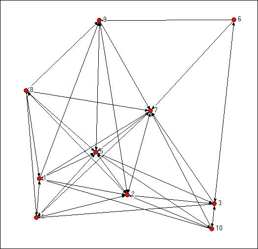
For small networks, it is often useful to examine graphs. Figure 7.1 shows the di-graph (directed graph) for the Knoke information exchange data:
Figure 7.1 Knoke information exchange directed graph

Your trained eye should immediately perceive a number of things in looking at the graph. There are a limited number of actors here (ten, actually), and all of them are "connected." But, clearly not every possible connection is present, and there are "structural holes" (or at least "thin spots" in the fabric). There appear to be some differences among the actors in how connected they are (compare actor number 7, a newspaper, to actor number 6, a welfare rights advocacy organization). If you look closely, you can see that some actor's connections are likely to be reciprocated (that is, if A shares information with B, B also shares information with A); some other actors (e.g. 6 and 10, are more likely to be senders than receivers of information). As a result of the variation in how connected individuals are, and whether the ties are reciprocated, some actors may be at quite some "distance" from other actors. There appear to be groups of actors who differ in this regard (2, 5, and 7 seem to be in the center of the action, 6, 9, and 10 seem to be more peripheral).
A careful look at the graph can be very useful in getting an intuitive grasp of the important features of a social network. With larger populations or more connections, however, graphs may not be much help. Looking at a graph can give a good intuitive sense of what is going on, but our descriptions of what we see are rather imprecise (the previous paragraph is an example of this). To get more precise, and to use computers to apply algorithms to calculate mathematical measures of graph properties, it is necessary to work with the adjacency matrix instead of the graph. The Knoke data graphed above are shown as an asymmetric adjacency matrix in figure 7.2.
Figure 7.2 Knoke information exchange adjacency matrix
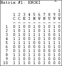
Using Data>Display, we can look at the network in matrix form. There are ten rows and columns, the data are binary, and the matrix is asymmetric. As we mentioned in the chapter on using matrices to represent networks, the row is treated as the source of information and the column as the receiver. By doing some very simple operations on this matrix it is possible to develop systematic and useful index numbers, or measures, of some of the network properties that our eye discerns in the graph.
Since networks are defined by their actors and the connections among them, it is useful to begin our description of networks by examining these very simple properties. Focusing first on the network as a whole, one might be interested in the number of actors, the number of connections that are possible, and the number of connections that are actually present. Differences in the size of networks, and how connected the actors are tell us two things about human populations that are critical. Small groups differ from large groups in many important ways -- indeed, population size is one of the most critical variables in all sociological analyses. Differences in how connected the actors in a population are may be a key indicator of the "cohesion," "solidarity," "moral density," and "complexity" of the social organization of a population.
Individuals, as well as whole networks, differ in these basic demographic features. Individual actors may have many or few ties. Individuals may be "sources" of ties, "sinks" (actors that receive ties, but don't send them), or both. These kinds of very basic differences among actors immediate connections may be critical in explaining how they view the world, and how the world views them. The number and kinds of ties that actors have are a basis for similarity or dissimilarity to other actors -- and hence to possible differentiation and stratification. The number and kinds of ties that actors have are keys to determining how much their embeddedness in the network constrains their behavior, and the range of opportunities, influence, and power that they have.
table of contentsNetwork size. The size of a network is often very important. Imagine a group of 12 students in a seminar. It would not be difficult for each of the students to know each of the others fairly well, and build up exchange relationships (e.g. sharing reading notes). Now imagine a large lecture class of 300 students. It would be extremely difficult for any student to know all of the others, and it would be virtually impossible for there to be a single network for exchanging reading notes. Size is critical for the structure of social relations because of the limited resources and capacities that each actor has for building and maintaining ties. Our example network has ten actors. Usually the size of a network is indexed simply by counting the number of nodes.
In any network there are (k * k-1) unique ordered pairs of actors (that is AB is different from BA, and leaving aside self-ties), where k is the number of actors. You may wish to verify this for yourself with some small networks. So, in our network of 10 actors, with directed data, there are 90 logically possible relationships. If we had undirected, or symmetric ties, the number would be 45, since the relationship AB would be the same as BA. The number of logically possible relationships then grows exponentially as the number of actors increases linearly. It follows from this that the range of logically possible social structures increases (or, by one definition, "complexity" increases) exponentially with size.
Actor degree. The number of actors places an upper limit on the number of connections that each individual can have (k-1). For networks of any size, though, few -- if any -- actors approach this limit. It can be quite useful to examine the distribution of actor degree. The distribution of how connected individual actors are can tell us a good bit about the social structure.
Since the data in our example are asymmetric (that is directed ties), we can distinguish between ties being sent and ties being received. Looking at the density for each row and for each column can tell us a good bit about the way in which actors are embedded in the overall density.
Tools>Univariate Stats provides quick summaries of the distribution of actor's ties.
Let's first examine these statistics for the rows, or out-degree of actors.
Figure 7.3. Dialog for Tools>Univariate Stats

Produces this result:
Figure 7.4. Out-degree statistics for Knoke information exchange
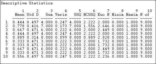
Statistics on the rows tell us about the role that each actor plays as a "source" of ties (in a directed graph). The sum of the connections from the actor to others (e.g. actor #1 sends information to four others) is called the out-degree of the point (for symmetric data, of course, each node simply has degree, as we cannot distinguish in-degree from out-degree). The degree of points is important because it tells us how many connections an actor has. With out-degree, it is usually a measure of how influential the actor may be.
We can see that actor #5 sends ties to all but one of the remaining actors; actors #6, #7 and #9 send information to only three other actors. Actors #2, #3, #5, and #8 are similar in being sources of information for large portions of the network; actors #1, #6, #7, and #9 as being similar as not being sources of information. We might predict that the first set of organizations will have specialized divisions for public relations, the latter set might not. Actors in the first set have a higher potential to be influential; actors in the latter set have lower potential to be influential; actors in "the middle" will be influential if they are connected to the "right" other actors, otherwise, they might have very little influence. So, there is variation in the roles that these organizations play as sources of information. We can norm this information (so we can compare it to other networks of different sizes, by expressing the out-degree of each point as a proportion of the number of elements in the row. That is, calculating the mean. Actor #10, for example, sends ties to 56% of the remaining actors. This is a figure we can compare across networks of different sizes.
Another way of thinking about each actor as a source of information is to look at the row-wise variance or standard deviation. We note that actors with very few out-ties, or very many out-ties have less variability than those with medium levels of ties. This tells us something: those actors with ties to almost everyone else, or with ties to almost no-one else are more "predictable" in their behavior toward any given other actor than those with intermediate numbers of ties. In a sense, actors with many ties (at the center of a network) and actors at the periphery of a network (few ties) have patterns of behavior that are more constrained and predictable. Actors with only some ties can vary more in their behavior, depending on to whom they are connected.
If we were examining a valued relation instead of a binary one, the meaning of the "sum," "mean," and "standard deviation" of actor's out-degree would differ. If the values of the relations are all positive and reflect the strength or probability of a tie between nodes, these statistics would have the easy interpretations as the sum of the strengths, the average strength, and variation in strength.
It's useful to examine the statistics for in-degree, as well (look at the data column-wise). Now, we are looking at the actors as "sinks" or receivers of information. The sum of each column in the adjacency matrix is the in-degree of the point. That is, how many other actors send information or ties to the one we are focusing on. Actors that receive information from many sources may be prestigious (other actors want to be known by the actor, so they send information). Actors that receive information from many sources may also be more powerful -- to the extent that "knowledge is power." But, actors that receive a lot of information could also suffer from "information overload" or "noise and interference" due to contradictory messages from different sources.
Here are the results of Tools>Univariate Stats when we select "column" instead of "row."
Figure7.5. In-degree statistics for Knoke information exchange
Looking at the means, we see that there is a lot of variation in information receiving -- more than for information sending. We see that actors #2, #5, and #7 are very high. #2 and #5 are also high in sending information -- so perhaps they act as "communicators" and "facilitators" in the system. Actor #7 receives a lot of information, but does not send a lot. Actor #7, as it turns out is an "information sink" -- it collects facts, but it does not create them (at least we hope so, since actor #7 is a newspaper). Actors #6, #8, and #10 appear to be "out of the loop" -- that is, they do not receive information from many sources directly. Actor #6 also does not send much information -- so #6 appears to be something of an "isolate." Numbers #8 and #10 send relatively more information than they receive. One might suggest that they are "outsiders" who are attempting to be influential, but may be "clueless."
We can learn a great deal about a network overall, and about the structural constraints on individual actors, and even start forming some hypotheses about social roles and behavioral tendencies, just by looking at the simple adjacencies and calculating a few very basic statistics. Before discussing the slightly more complex idea of distance, there are a couple other aspects of "connectedness" that are sometimes of interest.
The density of a binary network is simply the proportion of all possible ties that are actually present. For a valued network, density is defined as the sum of the ties divided by the number of possible ties (i.e. the ratio of all tie strength that is actually present to the number of possible ties). The density of a network may give us insights into such phenomena as the speed at which information diffuses among the nodes, and the extent to which actors have high levels of social capital and/or social constraint.
Network>Cohesion>Density is a quite powerful tool for calculating densities. its dialog is shown in figure 7.6.
Figure 7.6 Dialog for Network>Cohesion>Density
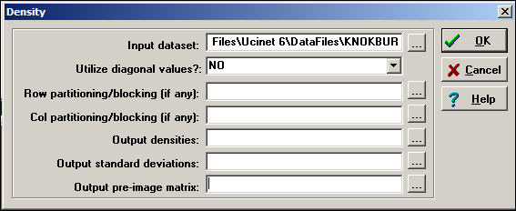
To obtain densities for a matrix (as we are doing in this example), we simply need a dataset. Usually self-ties are ignored in computing density (but there are circumstances where you might want to include them). The Network>Cohesion>Density algorithm also can be used to calculate the densities within partitions or blocks by specifying the file name of an attribute data set that contains the node name and partition number. That is, the density tool can be used to calculate within and between block densities for data that are grouped. One might, for example, partition the Knoke data into "public" and "private" organizations, and examine the density of information exchange within and between types.
For our current purposes, we won't block or partition the data. Here's the result of the dialog above.
Figure 7.7 Density of Knoke information network
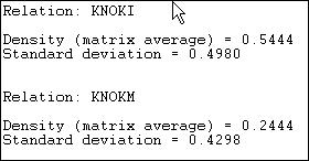
Since the Knoke data set contains two matrices, separate reports for each relation (KNOKI and KNOKM) are produced.
The density of the information exchange relation matrix is .5444. That is 54% of all the possible ties are present. The standard deviation of the entries in the matrix is also given. For binary data, the standard deviation is largely irrelevant -- as the standard deviation of a binary variable is a function of its mean.
An actor is "reachable" by another if there exists any set of connections by which we can trace from the source to the target actor, regardless of how many others fall between them. If the data are asymmetric or directed, it is possible that actor A can reach actor B, but that actor B cannot reach actor A. With symmetric or undirected data, of course, each pair of actors either are or are not reachable to one another. If some actors in a network cannot reach others, there is the potential of a division of the network. Or, it may indicate that the population we are studying is really composed of more than one sub-populations.
In the Knoke information exchange data set, it turns out that all actors are reachable by all others. This is something that you can verify by eye. See if you can find any pair of actors in the diagram such that you cannot trace from the first to the second along arrows all headed in the same direction (don't waste a lot of time on this, there is no such pair!). For the Knoke "M" relation, it turns out that not all actors can "reach" all other actors. Here's the output of Network>Cohesion>Reachability from UCINET.
Figure 7.8 Reachability of Knoke "I" and "M" relations
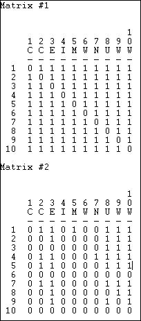
So, there exists a directed "path" from each organization to each other actor for the flow of information, but not for the flow of money. Sometimes "what goes around comes around," and sometimes it doesn't!
Adjacency tells us whether there is a direct connection from one actor to another (or between two actors for un-directed data). Reachability tells us whether two actors are connected or not by way of either a direct or an indirect pathways of any length.
Network>Cohesion>Point Connectivity calculates the number of nodes that would have to be removed in order for one actor to no longer be able to reach another. If there are many different pathways that connect two actors, they have high "connectivity" in the sense that there are multiple ways for a signal to reach from one to the other. Figure 7.9 shows the point connectivity for the flow information among the 10 Knoke organizations.
Figure 7.9. Point connectivity of Knoke information exchange
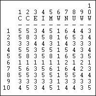
The result again demonstrates the tenuousness of organization 6's connection as both a source (row) or receiver (column) of information. To get its message to most other actors, organization 6 has alternative; should a single organization refuse to pass along information, organization 6 would receive none at all! Point connectivity can be a useful measure to get at notions of dependency and vulnerability.
The properties of the network that we have examined so far primarily deal with adjacencies -- the direct connections from one actor to the next. But the way that people are embedded in networks is more complex than this. Two persons, call them A and B, might each have five friends. But suppose that none of person A's friends have any friends except A. Person B's five friends, in contrast, each have five friends. The information available to B, and B's potential for influence is far greater than A's. That is, sometimes being a "friend of a friend" may be quite consequential.
To capture this aspect of how individuals are embedded in networks, one main approach is to examine the distance that an actor is from others. If two actors are adjacent, the distance between them is one (that is, it takes one step for a signal to go from the source to the receiver). If A tells B, and B tells C (and A does not tell C), then actors A and C are at a distance of two. How many actors are at various distances from each actor can be important for understanding the differences among actors in the constraints and opportunities they have as a result of their position. Sometimes we are also interested in how many ways there are to connect between two actors, at a given distance. That is, can actor A reach actor B in more than one way? Sometimes multiple connections may indicate a stronger connection between two actors than a single connection.
The distances among actors in a network may be an important macro-characteristic of the network as a whole. Where distances are great, it may take a long time for information to diffuse across a population. It may also be that some actors are quite unaware of, and influenced by others -- even if they are technically reachable, the costs may be too high to conduct exchanges. The variability across the actors in the distances that they have from other actors may be a basis for differentiation and even stratification. Those actors who are closer to more others may be able to exert more power than those who are more distant. We will have a good deal more to say about this aspect of variability in actor distances in the next chapter.
For the moment, we need to learn a bit of jargon that is used to describe the distances between actors: walks, paths, semi-paths, etc. Using these basic definitions, we can then develop some more powerful ways of describing various aspects of the distances among actors in a network.
To describe the distances between actors in a network with precision, we need some terminology. And, as it turns out, whether we are talking about a simple graph or a directed graph makes a good bit of difference. If A and B are adjacent in a simple graph, they have a distance of one. In a directed graph, however, A can be adjacent to B while B is not adjacent to A -- the distance from A to B is one, but there is no distance from B to A. Because of this difference, we need slightly different terms to describe distances between actors in graphs and digraphs.
Simple graphs: The most general form of connection between two actors in a graph is called a walk. A walk is a sequence of actors and relations that begins and ends with actors. A closed walk is one where the beginning and end point of the walk are the same actor. Walks are unrestricted. A walk can involve the same actor or the same relation multiple times. A cycle is a specially restricted walk that is often used in algorithms examining the neighborhoods (the points adjacent) of actors. A cycle is a closed walk of 3 or more actors, all of whom are distinct, except for the origin/destination actor. The length of a walk is simply the number of relations contained in it. For example, consider this graph in figure 7.10.
Figure 7.10. Walks in a simple graph
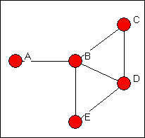
There are many walks in a graph (actually, an infinite number if we are willing to include walks of any length -- though, usually, we restrict our attention to fairly small lengths). To illustrate just a few, begin at actor A and go to actor C. There is one walk of length 2 (A,B,C). There is one walk of length three (A,B,D,C). There are several walks of length four (A,B,E,D,C; A,B,D,B,C; A,B,E,B,C). Because these are unrestricted, the same actors and relations can be used more than once in a given walk. There are no cycles beginning and ending with A. There are some beginning and ending with actor B (B,D,C,B; B,E,D,B; B,C,D,E,B).
It is usually more useful to restrict our notion of what constitutes a connection somewhat. One possibility is to restrict the count only walks that do not re-use relations. A trail between two actors is any walk that includes a given relation no more than once (the same other actors, however, can be part of a trail multiple times. The length of a trail is the number of relations in it. All trails are walks, but not all walks are trails. If the trail begins and ends with the same actor, it is called a closed trail. In our example above, there are a number of trails from A to C. Excluded are tracings like A,B,D,B,C (which is a walk, but is not a trail because the relation BD is used more than once).
Perhaps the most useful definition of a connection between two actors (or between an actor and themself) is a path. A path is a walk in which each other actor and each other relation in the graph may be used at most one time. The single exception to this is a closed path, which begins and ends with the same actor. All paths are trails and walks, but all walks and all trails are not paths. In our example, there are a limited number of paths connecting A and C: A,B,C; A,B,D,C; A,B,E,D,C.
Directed graphs: Walks, trails, and paths can also be defined for directed graphs. But there are two flavors of each, depending on whether we want to take direction into account or not . Semi-walks, semi-trails, and semi-paths are the same as for undirected data. In defining these distances, the directionality of connections is simply ignored (that is, arcs - or directed ties are treated as though they were edges - undirected ties). As always, the length of these distances is the number of relations in the walk, trail, or path.
If we do want to pay attention to the directionality of the connections we can define walks, trails, and paths in the same way as before, but with the restriction that we may not "change direction" as we move across relations from actor to actor. Consider the directed graph in figure 7.11
Figure 7.11. Walks in a directed graph
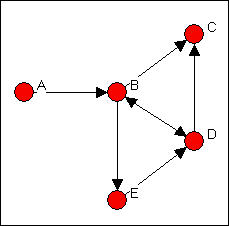
In this directed graph, there are a number of walks from A to C. However, there are no walks from C (or anywhere else) to A. Some of these walks from A to C are also trails (e.g. A,B,E,D,B,C). There are, however, only three paths from A to C. One path is length 2 (A,B,C); one is length three (A,B,D,C); one is length four (A,B,E,D,C).
The various kinds of connections (walks, trails, paths) provide us with a number of different ways of thinking about the distances between actors. The main reason that social network analysts are concerned with these distances is that they provide a way of thinking about the strength of ties or relations. Actors that are connected at short lengths or distances may have stronger connections; actors that are connected many times (for example, having many, rather than a single path) may have stronger ties. Their connection may also be less subject to disruption, and hence more stable and reliable.
The numbers of walks of a given length between all pairs of actors can be found by raising the matrix to that power. A convenient method for accomplishing this is to use Tools>Matrix Algebra, and to specify an expression like out=prod(X1,X1). This produces the square of the matrix X1, and stores it as the data set "out." A more detailed discussion of this idea can be found in the earlier chapter on representing networks as matrices. This matrix could then be added to X1 to show the number of walks between any two actors of length two or less.
Let's look briefly at the distances between pairs of actors in the Knoke data on directed information flows. Counts of the numbers of paths of various lengths are shown in figure 7.12.
Figure 7.12. Numbers of walks in Knoke information network
# of walks of length 1
                       1
     1 2 3 4 5 6 7 8 9 0
     - - - - - - - - - -
  1  0 1 0 0 1 0 1 0 1 0
  2  1 0 1 1 1 0 1 1 1 0
  3  0 1 0 1 1 1 1 0 0 1
  4  1 1 0 0 1 0 1 0 0 0
  5  1 1 1 1 0 0 1 1 1 1
  6  0 0 1 0 0 0 1 0 1 0
  7  0 1 0 1 1 0 0 0 0 0
  8  1 1 0 1 1 0 1 0 1 0
  9  0 1 0 0 1 0 1 0 0 0
 10  1 1 1 0 1 0 1 0 0 0

# of walks of length 2
                       1
     1 2 3 4 5 6 7 8 9 0
     - - - - - - - - - -
  1  2 3 2 3 3 0 3 2 2 1
  2  3 7 1 4 6 1 6 1 3 2
  3  4 4 4 3 4 0 5 2 3 1
  4  2 3 2 3 3 0 3 2 3 1
  5  4 7 2 4 8 1 7 1 3 1
  6  0 3 0 2 3 1 2 0 0 1
  7  3 2 2 2 2 0 3 2 2 1
  8  3 5 2 3 5 0 5 2 3 1
  9  2 2 2 3 2 0 2 2 2 1
 10  2 4 2 4 4 1 4 2 3 2

# of walks of length 3
      1  2  3  4  5  6  7  8  9 10
     -- -- -- -- -- -- -- -- -- --
  1  12 18  7 13 18  2 18  6 10  5
  2  20 26 16 21 27  1 28 13 18  7
  3  14 26  9 19 26  4 25  8 14  8
  4  12 19  7 13 19  2 19  6 10  5
  5  21 30 17 25 29  2 31 15 21 10
  6   9  8  8  8  8  0 10  6  7  3
  7   9 17  5 11 17  2 16  4  9  4
  8  16 24 11 19 24  2 24 10 15  7
  9  10 16  5 10 16  2 16  4  8  4
 10  16 23 11 16 23  2 24  8 13  6

Total number of walks (lengths 1, 2, 3)
       1  2  3  4  5  6  7  8  9 10
      -- -- -- -- -- -- -- -- -- --
  1   14 21  9 16 21  2 21  8 12  6
  2   23 33 17 25 33  2 34 14 21  9
  3   18 30 13 22 30  4 30 10 17  9
  4   14 22  9 16 22  2 22  8 13  6
  5   25 37 19 29 37  3 38 16 24 11
  6    9 11  8 10 11  1 12  6  7  4
  7   12 19  7 13 19  2 19  6 11  5
  8   19 29 13 22 29  2 29 12 18  8
  9   12 18  7 13 18  2 18  6 10  5
 10   18 27 13 20 27  3 28 10 16  8
The inventory of the total connections among actors is primarily useful for getting a sense of how "close" each pair is, and for getting a sense of how closely coupled the entire system is. Here, we can see that using only connections of two steps (e.g. "A friend of a friend"), there is a great deal of connection in the graph overall; we also see that there are sharp differences among actors in their degree of connectedness, and who they are connected to. These differences can be used to understand how information moves in the network, which actors are likely to be influential on one another, and a number of other important properties.
One particular definition of the distance between actors in a network is used by most algorithms to define more complex properties of individual's positions and the structure of the network as a whole. This quantity is the geodesic distance. For both directed and undirected data, the geodesic distance is the number of relations in the shortest possible walk from one actor to another (or, from an actor to themselves, if we care, which we usually do not).
The geodesic distance is widely used in network analysis. There may be many connections between two actors in a network. If we consider how the relation between two actors may provide each with opportunity and constraint, it may well be the case that not all of these ties matter. For example, suppose that I am trying to send a message to Sue. Since I know her e-mail address, I can send it directly (a path of length 1). I also know Donna, and I know that Donna has Sue's email address. I could send my message for Sue to Donna, and ask her to forward it. This would be a path of length two. Confronted with this choice, I am likely to choose the geodesic path (i.e. directly to Sue) because it is less trouble and faster, and because it does not depend on Donna. That is, the geodesic path (or paths, as there can be more than one) is often the "optimal" or most "efficient" connection between two actors. Many algorithms in network analysis assume that actors will use the geodesic path when alternatives are available.
Using UCINET, we can easily locate the lengths of the geodesic paths in our directed data on information exchanges. Here is the dialog box for Network>Cohesion>Distance.
Figure 7.13. Network>Cohesion>Distance dialog
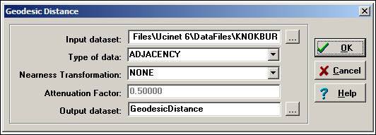
The Knoke information exchange data are binary (organization A sends information to organization B, or it doesn't). That is, the pattern is summarized by an adjacency matrix. For binary data, the geodesic distance between two actors is the count of the number of links in the shortest path between them.
It is also possible to define the distance between two actors where the links are valued. That is, where we have a measure of the strength of ties, the opportunity costs of ties, or the probability of a tie. Network>Cohesion>Distance can calculate distance (and nearness) for valued data, as well (select the appropriate "type of data").
Where we have measures of the strengths of ties (e.g. the dollar volume of trade between two nations), the "distance" between two actors is defined as the strength of the weakest path between them. If A sends 6 units to B, and B sends 4 units to C, the "strength" of the path from A to C (assuming A to B to C is the shortest path) is 4.
Where we have a measure of the cost of making a connection (as in an "opportunity cost" or "transaction cost" analysis), the "distance" between two actors is defined as the sum of the costs along the shortest pathway.
Where we have a measure of the probability that a link will be used, the "distance" between two actors is defined as the product along the pathway -- as in path analysis in statistics.
The Nearness Transformation and Attenuation Factor parts of the dialog allow the rescaling of distances into near-nesses. For many analyses, we may be interesting in thinking about the connections among actors in terms of how close or similar they are, rather than how distant. There are a number of ways that this may be done.
The multiplicative nearness transformation divides the distance by the largest possible distance between two actors. For example, if we had 7 nodes, the maximum possible distance for adjacency data would be 6. This method gives a measure of the distance as a percentage of the theoretical maximum for a given graph.
The additive nearness transformation subtracts the actual distance between two actors from the number of nodes. It is similar to the multiplicative scaling, but yields a value as the nearness measure, rather than a proportion.
The linear nearness transformation rescales distance by reversing the scale (i.e. the closest becomes the most distant, the most distant becomes the nearest) and re-scoring to make the scale range from zero (closest pair of nodes) to one (most distant pair of nodes).
The exponential decay method turns distance into nearness by weighting the links in the pathway with decreasing values as they fall farther away from ego. With an attenuation factor of .5, for example, a path from A to B to C would result in a distance of 1.5.
The frequency decay method is defined as 1 minus the proportion of other actors who are as close or closer to the target as ego is. The idea (Ron Burt's) is that if there are many other actors closer to the target you are trying to reach than yourself, you are effectively "more distant."
In our example, we are using simple directed adjacencies, and the results (figure 7.14) are quite straight-forward.
Figure 7.14. Geodesic distances for Knoke information exchange
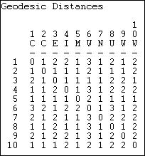
Because the network is moderately dense, the geodesic distances are generally small. This suggests that information may travel pretty quickly in this network. Also note that there is a geodesic distance for each x, y and y, x pair -- that is, the graph is fully connected, and all actors are "reachable" from all others (that is, there exists a path of some length from each actor to each other actor). When a network is not fully connected, we cannot exactly define the geodesic distances among all pairs. The standard approach in such cases is to treat the geodesic distance between unconnected actors as a length greater than that of any real distance in the data. For each actor, we could calculate the mean and standard deviation of their geodesic distances to describe their closeness to all other actors. For each actor, that actor's largest geodesic distance is called the eccentricity -- a measure of how far a actor is from the furthest other.
Because the current network is fully connected, a message that starts anywhere will eventually reach everyone. Although the computer has not calculated it, we might want to calculate the mean (or median) geodesic distance, and the standard deviation in geodesic distances for the matrix, and for each actor row-wise and column-wise. This would tell us how far each actor is from each other as a source of information for the other; and how far each actor is from each other actor who may be trying to influence them. It also tells us which actors behavior (in this case, whether they've heard something or not) is most predictable and least predictable.
In looking at the whole network, we see that it is connected, and that the average geodesic distance among actors is quite small. This suggests a system in which information is likely to reach everyone, and to do so fairly quickly. To get another notion of the size of a network, we might think about its diameter. The diameter of a network is the largest geodesic distance in the (connected) network. In the current case, no actor is more than three steps from any other -- a very "compact" network. The diameter of a network tells us how "big" it is, in one sense (that is, how many steps are necessary to get from one side of it to the other). The diameter is also a useful quantity in that it can be used to set an upper bound on the lengths of connections that we study. Many researchers limit their explorations of the connections among actors to involve connections that are no longer than the diameter of the network.
Sometimes the redundancy of connection is an important feature of a network structure. If there are many efficient paths connecting two actors, the odds are improved that a signal will get from one to the other. One index of this is a count of the number of geodesic paths between each pair of actors. Of course, if two actors are adjacent, there can only be one such path. The number of geodesic paths can be calculated with Network>Cohesion>No. of Geodesics, as in figure 7.15.
Figure 7.15. Dialog for Network>Cohesion>No. of Geodesics

The results are shown in figure 7.16.
Figure 7.16. Number of geodesic paths for Knoke information exchange
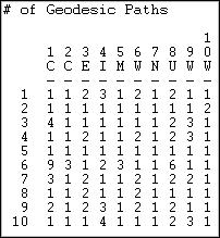
We see that most of the geodesic connections among these actors are not only short distance, but that there are very often multiple shortest paths from x to y. This suggests a couple things: information flow is not likely to break down, because there are multiple paths; and, it will be difficult for any individual to be a powerful "broker" in this structure because most actors have alternative efficient ways of connection to other actors that can by-pass any given actor.
The use of geodesic paths to examine properties of the distances between individuals and for the whole network often makes a great deal of sense. But, there may be other cases where the distance between two actors, and the connectedness of the graph as a whole is best thought of as involving all connections -- not just the most efficient ones. If I start a rumor, for example, it will pass through a network by all pathways -- not just the most efficient ones. How much credence another person gives my rumor may depend on how many times they hear it form different sources -- and not how soon they hear it. For uses of distance like this, we need to take into account all of the connections among actors.
Several approaches have been developed for counting the amount of connection between pairs of actors that take into account all connections between them. These measures have been used for a number of different purposes, and these differences are reflected in the algorithms used to calculate them. We will examine three such ideas.
Network>Cohesion>Maximum Flow. One notion of how totally connected two actors are (called maximum flow by UCINET) asks how many different actors in the neighborhood of a source lead to pathways to a target. If I need to get a message to you, and there is only one other person to whom I can send this for retransmission, my connection is weak - even if the person I send it to may have many ways of reaching you. If, on the other hand, there are four people to whom I can send my message, each of whom has one or more ways of retransmitting my message to you, then my connection is stronger. The "flow" approach suggests that the strength of my tie to you is no stronger than the weakest link in the chain of connections, where weakness means a lack of alternatives. This approach to connection between actors is closely connected to the notion of between-ness that we will examine a bit later. It is also logically close to the idea that the number of pathways, not their length may be important in connecting people. For our directed information flow data, the results of UCINET's count of maximum flow are shown in figure 7.17.
Figure 7.17. Maximum flow for Knoke information network
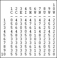
You should verify for yourself that, for example, there are four intermediaries, or alternative routes in flows from actor 1 to actor 2, but five such points in the flow from actor 2 to actor 1. The higher the number of flows from one actor to another, the greater the likelihood that communication will occur, and the less "vulnerable" the connection. Note that actors 6, 7, and 9 are relatively disadvantaged. In particular, actor 6 has only one way of obtaining information from all other actors (the column vector of flows to actor 6).
There is a great deal of information about both individuals and the population in a single adjacency matrix. In this chapter you have learned a lot of terminology for describing the connections and distances between actors, and for whole populations.
One focus in basic network analysis is on the immediate neighborhood of each actor: the dyads and triads in which they are involved. The degree of an actor, and the in-degree and out-degree (if the data are directed) tell us about the extent to which an actor may be constrained by, or constrain others. The extent to which an actor can reach others in the network may be useful in describing an actor's opportunity structure. We have also seen that it is possible to describe "types" of actors who may form groups or strata on the basis of their places in opportunity structures -- e.g. "isolates" "sources" etc.
Most of the time and effort of most social actors is spent in very local contexts -- interacting in dyads and triads. In looking at the connections of actors, we have suggested that the degree of "reciprocity" and "balance" and "transitivity" in relations can be regarded as important indicators of the stability and institutionalization (that is, the extent to which relations are taken for granted and are norm governed) of actor's positions in social networks.
The local connections of actors are important for understanding the social behavior of the whole population, as well as for understanding each individual. The size of the network, its density, whether all actors are reachable by all others (i.e. is the whole population connected, or are there multiple components?), whether ties tend to be reciprocal or transitive, and all the other properties that we examined for individual connections are meaningful in describing the whole population. Both the typical levels of characteristics (e.g. the mean degree of points), and the amount of diversity in characteristics (e.g. the variance in the degree of points) may be important in explaining macro behavior. Populations with high density respond differently to challenges from the environment than those with low density; populations with greater diversity in individual densities may be more likely to develop stable social differentiation and stratification.
In this chapter we also examined some properties of individual's embeddedness and of whole networks that look at the broader, rather than the local neighborhoods of actors. A set of specialized terminology was introduced to describe the distances between pairs of actors: walks, trails, and paths. We noted that there are some important differences between un-directed and directed data in applying these ideas of distance.
One of the most common and important approaches to indexing the distances between actors is the geodesic. The geodesic is useful for describing the minimum distance between actors. The geodesic distances between pairs of actors is the most commonly used measure of closeness. The average geodesic distance for an actor to all others, the variation in these distances, and the number of geodesic distances to other actors may all describe important similarities and differences between actors in how, and how closely they are connected to their entire population.
The geodesic distance, however, examines only a single connection between a pair of actors (or, in some cases several, if there are multiple geodesics connecting them). Sometimes the sum of all connections between actors, rather than the shortest connection may be relevant. We have examined approaches to measuring the vulnerability of the connection between actors by looking at the number of geodesic connections between pairs of actors, and the total number of pathways between pairs of actors.
We have seen that there is a great deal of information available in fairly simple examinations of an adjacency matrix. Life, of course, can get more complicated. We could have multiple layers, or multiplex data; we could have data that gave information on the strength of ties, rather than simple presence or absence. Nonetheless, the methods that we've used here will usually give you a pretty good grasp of what is going on in more complicated data.
Now that you have a pretty good grasp of the basics of connection and distance, you are ready to use these ideas to build some concepts and methods for describing somewhat more complicated aspects of the network structures of populations. In the next two chapters, we will focus on ways of examining the local neighborhoods of actors. In chapter 8, we will look at methods for summarizing the entire graph in terms of the kinds of connections that individuals have to their neighbors. In chapter 9, we'll examine actors local neighborhoods from their own individual perspective.
1. Explain the differences among the "three levels of analysis" of graphs (individual, aggregate, whole).
2. How is the size of a network measured? Why is population size so important is sociological analysis?
3. You have a network of 5 actors, assuming no self-ties, what is the potential number of directed ties? what is the potential number of un-directed ties?
4. How is density measured? Why is density important is sociological analysis?
5. What is the "degree of a point?" Why might it be important, sociologically, if some actors have high degree and other actors have lower degree? What is the difference between "in-degree" and "out-degree?"
6. If actor "A" is reachable from actor "B" does that necessarily mean that actor "B" is reachable from actor "A?" Why or why not?
7. For pairs of actors with directed relations, there are four possible configurations of ties. Can you show these? Which configurations are "balanced?" For a triad with undirected relations, how many possible configurations of ties are there? which ones are balanced or transitive?
8. What are the differences among walks, trails, and paths? Why are "paths" the most commonly used approach to inter-actor distances in sociological analysis?
9. What is the "geodesic" distance between two actors? Many social network measures assume that the geodesic path is the most important path between actors -- why is this a plausible assumption?
10. I have two populations of ten actors each, one has a network diameter of 3, the other has a network diameter of 6. Can you explain this statement to someone who doesn't know social network analysis? Can you explain why this difference in diameter might be important in understanding differences between the two populations?
11. How do "weighted flow" approaches to social distance differ from "geodesic" approaches to social distance?
12. Why might it matter if two actors have more than one geodesic or other path between them?
Application questions
1. Think of the readings from the first part of the course. Which studies used the ideas of connectedness and density? Which studies used the ideas of distance? What specific approaches did they use to measure these concepts?
2. Draw the graphs of a "star" a "circle" a "line" and a "hierarchy." Describe the size, potential, and density of each graph. Examine the degrees of points in each graph -- are there differences among actors? Do these differences tell us something about the "social roles" of the actors? Create a matrix for each graph that shows the geodesic distances between each pair of actors. Are there differences between the graphs in whether actors are connected by mulitple geodesic distances?
3. Think about a small group of people that you know well (maybe your family, neighbors, a study group, etc.). Who helps whom in this group? What is the density of the ties? Are ties reciprocated? Are triads transitive?
4. Chrysler Corporation has called on you to be a consultant. Their research division is taking too long to generate new models of cars, and often the work of the "stylists" doesn't fit well with the work of the "manufacturing engineers" (the people who figure out how to actually build the car). Chrysler's research division is organized as a classical hierarchical bureaucracy with two branches (stylists, manufacturing) coordinated through group managers and a division manager. Analyze the reasons why performance is poor. Suggest some alternative ways of organizing that might improve performance, and explain why they will help.