18. Some statistical tools
Network analysis in the social sciences developed from a conjuncture of anthropologist's observations about relations in face-to-face groups and mathematical graph theory. A very large part of social network methodology, consequently, deals with relatively small networks, networks where we have confidence in the reliability of our observations about the relations among the actors. Most of the tools of social network analysis involve the use of mathematical functions to describe networks and their sub-structures.
In more recent work, however, some of the focus of social network research has moved away from these roots. Increasingly, the social networks that are being studied may contain many nodes; and, sometimes our observations about these very large networks are based not on censuses, but on samples of nodes. Network researchers have come to recognize that the relations that they study may be constantly evolving, and that the relations observed at one point in time may not the entirely typical because the pattern of relations is not "in equilibrium." They have also recognized that sometimes our observations are fallible -- we fail to record a relation that actually exists, or mis-measure the strength of a tie.
All of these concerns (large networks, sampling, concern about the reliability of observations) have led social network researchers to begin to apply the techniques of descriptive and inferential statistics in their work. Statistics provide useful tools for summarizing large amounts of information, and for treating observations as stochastic, rather than deterministic outcomes of social processes.
Descriptive statistics have proven to be of great value because they provide convenient tools to summarize key facts about the distributions of actors, attributes, and relations; statistical tools can describe not only the shape of one distribution, but also joint distributions, or "statistical association." So, statistical tools have been particularly helpful in describing, predicting, and testing hypotheses about the relations between network properties.
Inferential statistics have also proven to have very useful applications to social network analysis. At a most general level, the question of "inference" is: how much confidence can I have that the pattern I see in the data I've collected is actually typical of some larger population, or that the apparent pattern is not really just a random occurrence?
In this chapter we will look at some of the ways in which quite basic statistical tools have been applied in social network analysis. These are only the starting point. The development of more powerful statistical tools especially tuned for the needs of social network analysis is one of the most rapidly developing "cutting edges" of the field.
table of contentsMost social scientists have a reasonable working knowledge of basic univariate and bivariate descriptive and inferential statistics. Many of these tools find immediate application in working with social network data. There are, however, two quite important distinctive features of applying these tools to network data.
First, and most important, social network analysis is about relations among actors, not about relations between variables. Most social scientists have learned their statistics with applications to the study of the distribution of the scores of actors (cases) on variables, and the relations between these distributions. We learn about the mean of a set of scores on the variable "income." We learn about the Pearson zero-order product moment correlation coefficient for indexing linear association between the distribution of actor's incomes and actor's educational attainment.
The application of statistics to social networks is also about describing distributions and relations among distributions. But, rather than describing distributions of attributes of actors (or "variables"), we are concerned with describing the distributions of relations among actors. In applying statistics to network data, we are concerned the issues like the average strength of the relations between actors; we are concerned with questions like "is the strength of ties between actors in a network correlated with the centrality of the actors in the network?" Most of the descriptive statistical tools are the same for attribute analysis and for relational analysis -- but the subject matter is quite different!
Second, many of tools of standard inferential statistics that we learned from the study of the distributions of attributes do not apply directly to network data. Most of the standard formulas for calculating estimated standard errors, computing test statistics, and assessing the probability of null hypotheses that we learned in basic statistics don't work with network data (and, if used, can give us "false positive" answers more often than "false negative"). This is because the "observations" or scores in network data are not "independent" samplings from populations. In attribute analysis, it is often very reasonable to assume that Fred's income and Fred's education are a "trial" that is independent of Sue's income and Sue's education. We can treat Fred and Sue as independent replications.
In network analysis, we focus on relations, not attributes. So, one observation might well be Fred's tie with Sue; another observation might be Fred's tie with George; still another might be Sue's tie with George. These are not "independent" replications. Fred is involved in two observations (as are Sue an George), it is probably not reasonable to suppose that these relations are "independent" because they both involve George.
The standard formulas for computing standard errors and inferential tests on attributes generally assume independent observations. Applying them when the observations are not independent can be very misleading. Instead, alternative numerical approaches to estimating standard errors for network statistics are used. These "boot-strapping" (and permutations) approaches calculate sampling distributions of statistics directly from the observed networks by using random assignment across hundreds or thousands of trials under the assumption that null hypotheses are true.
These general points will become clearer as we examine some real cases. So, let's begin with the simplest univariate descriptive and inferential statistics, and then move on to somewhat more complicated problems.
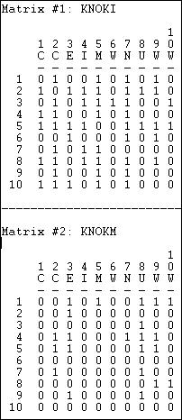
table of contentsFor most of the examples in this chapter, we'll focus again on the Knoke data set that describes the two relations of the exchange of information and the exchange of money among ten organizations operating in the social welfare field. Figure 18.1 lists these data.
Figure 18.1. Listing (Data>Display) of Knoke information and money exchange matrices

These particular data happen to be asymmetric and binary. Most of the statistical tools for working with network data can be applied to symmetric data, and data where the relations are valued (strength, cost, probability of a tie). As with any descriptive statistics, the scale of measurement (binary or valued) does matter in making proper choices about interpretation and application of many statistical tools.
The data that are analyzed with statistical tools when we are working with network data are the observations about relations among actors. So, in each matrix, we have 10 x 10 = 100 observations or cases. For many analyses, the ties of actors with themselves (the main diagonal) are not meaningful, and are not used, so there would be (N * N-1= 90) observations. If data are symmetric (i.e. Xij = Xji), half of these are redundant, and wouldn't be used, so there would be (N * N-1 / 2 = 45) observations.
What we would like to summarize with our descriptive statistics are some characteristics of the distribution of these scores. Tools>Univariate Stats can be used to generate the most commonly used measures for each matrix (select matrix in the dialog, and chose whether or not to include the diagonal). Figure 18.2 shows the results for our example data, excluding the diagonal.
Figure 18.2. Univariate descriptive statistics for Knoke information and money whole networks
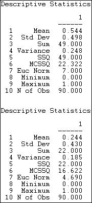
For the information sharing relation, we see that we have 90 observations which range from a minimum score of zero to a maximum of one. The sum of the ties is 49, and the average value of the ties is 49/90 = .544. Since the relation has been coded as a "dummy" variable (zero for no relation, one for a relation) the mean is also the proportion of possible ties that are present (or the density), or the probability that any given tie between two random actors is present (54.4% chance).
Several measures of the variability of the distribution are also given. The sums of squared deviations from the mean, variance, and standard deviation are computed -- but are more meaningful for valued than binary data. The Euclidean norm (which is the square root of the sum of squared values) is also provided. One measure not given, but sometimes helpful is the coefficient of variation (standard deviation / mean times 100) equals 91.5. This suggests quite a lot of variation as a percentage of the average score. No statistics on distributional shape (skew or kurtosis) are provided by UCINET.
A quick scan tells us that the mean (or density) for money exchange is lower, and has slightly less variability.
In addition to examining the entire distribution of ties, we might want to examine the distribution of ties for each actor. Since the relation we're looking at is asymmetric or directed, we might further want to summarize each actor's sending (row) and receiving (column). Figures 18.3 and 18.4 show the results of Tools>Univariate Stats for rows (tie sending) and columns (tie receiving) of the information relation matrix.
Figure 18.3. Univariate descriptive statistics for Knoke information network rows
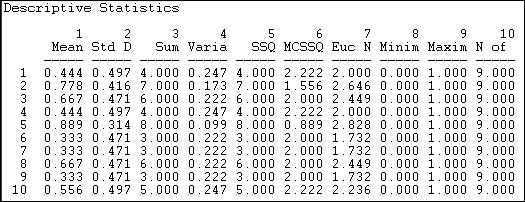
Figure 18.4. Univariate descriptive statistics for Knoke information network columns
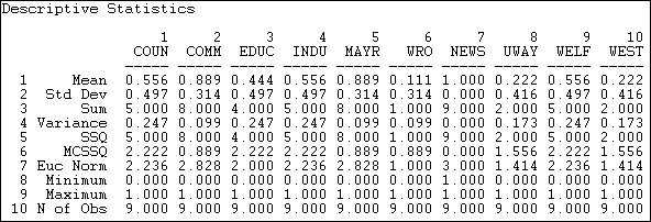
We see that actor 1 (COUN) has a mean (or density) of tie sending of .444. That is, this actor sent four ties to the available nine other actors. Actor 1 received somewhat more information than they sent, as their column mean is .556. In scanning down the column (in figure 18.3) or row (in figure 18.4) of means, we note that there is quite a bit of variability across actors -- some send more and get more information than others.
With valued data, the means produced index the average strength of ties, rather than the probability of ties. With valued data, measures of variability may be more informative than they are with binary data (since the variability of a binary variable is strictly a function of its mean).
The main point of this brief section is that when we use statistics to describe network data, we are describing properties of the distribution of relations, or ties among actors -- rather than properties of the distribution of attributes across actors. The basic ideas of central tendency and dispersion of distributions apply to the distributions of relational ties in exactly the same way that they do to attribute variables -- but we are describing relations, not attributes.
table of contentsOf the various properties of the distribution of a single variable (e.g. central tendency, dispersion, skewness), we are usually most interested in central tendency.
If we are working with the distribution of relations among actors in a network, and our measure of tie-strength is binary (zero/one), the mean or central tendency is also the proportion of all ties that are present, and is the "density."
If we are working with the distribution of relations among actors in a network, and our measure of tie-strength is valued, central tendency is usually indicated by the average strength of the tie across all the relations.
We may want to test hypotheses about the density or mean tie strength of a network. In the analysis of variables, this is testing a hypothesis about a single-sample mean or proportion. We might want to be confident that there actually are ties present (null hypothesis: network density is really zero, and any deviation that we observe is due to random variation). We might want to test the hypothesis that the proportion of binary ties present differs from .50; we might want to test the hypothesis that the average strength of a valued tie differs from "3."
Network>Compare densities>Against theoretical parameter performs a statistical test to compare the value of a density or average tie strength observed in a network against a test value.
Let's suppose that I think that all organizations have a tendency to want to directly distribute information to all others in their field as a way of legitimating themselves. If this theory is correct, then the density of Knoke's information network should be 1.0. We can see that this isn't true. But, perhaps the difference between what we see (density = .544) and what the theory predicts (density = 1.000) is due to random variation (perhaps when we collected the information).
The dialog in figure 18.5 sets up the problem.
Figure 18.5. Dialog of Compare densities>Against theoretical parameter

The "Expected density" is the value against which we want to test. Here, we are asking the data to convince us that we can be confident in rejecting the idea that organizations send information to all others in their fields.
The parameter "Number of samples" is used for estimating the standard error for the test by the means of "bootstrapping" or computing estimated sampling variance of the mean by drawing 5000 random sub-samples from our network, and constructing a sampling distribution of density measures. The sampling distribution of a statistic is the distribution of the values of that statistic on repeated sampling. The standard deviation of the sampling distribution of a statistic (how much variation we would expect to see from sample to sample just by random chance) is called the standard error. Figure 18.6 shows the results of the hypothesis test
Figure 18.6. Test results
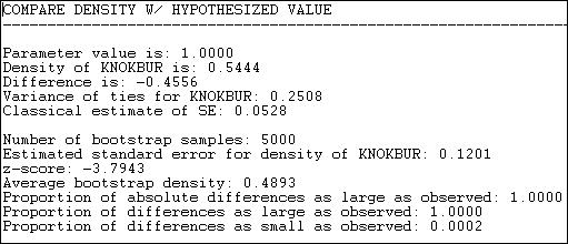
We see that our test value was 1.000, the observed value was .5444, so the difference between the null and observed values is -.4556. How often would a difference this large happen by random sampling variation, if the null hypothesis (density = 1.000) was really true in the population?
Using the classical formula for the standard error of a mean (s / sqr(N)) we obtain a sampling variability estimate of .0528. If we used this for our test, the test statistic would be -.4556//.0528 = 8.6 which would be highly significant as a t-test with N-1 degrees of freedom.
However, if we use the bootstrap method of constructing 5000 networks by sampling random sub-sets of nodes each time, and computing the density each time, the mean of this sampling distribution turns out to be .4893, and its standard deviation (or the standard error) turns out to be .1201.
Using this alternative standard error based on random draws from the observed sample, our test statistic is -3.7943. This test is also significant (p = .0002).
Why do this? The classical formula gives an estimate of the standard error (.0528) that is much smaller than than that created by the bootstrap method (.1201). This is because the standard formula is based on the notion that all observations (i.e. all relations) are independent. But, since the ties are really generated by the same 10 actors, this is not a reasonable assumption. Using the actual data on the actual actors -- with the observed differences in actor means and variances, is a much more realistic approximation to the actual sampling variability that would occur if, say, we happened to miss Fred when we collected the data on Tuesday.
In general, the standard inferential formulas for computing expected sampling variability (i.e. standard errors) give unrealistically small values for network data. Using them results in the worst kind of inferential error -- the false positive, or rejecting the null when we shouldn't.
table of contentsThe basic question of bivariate descriptive statistics applied to variables is whether scores on one attribute align (co-vary, correlate) with scores on another attribute, when compared across cases. The basic question of bivariate analysis of network data is whether the pattern of ties for one relation among a set of actors aligns with the pattern of ties for another relation among the same actors. That is, do the relations correlate?
Three of the most common tools for bivariate analysis of attributes can also be applied to the bivariate analysis of relations:
Does the central tendency of one relation differ significantly from the central tendency of another? For example, if we had two networks that described the military and the economic ties among nations, which has the higher density? Are military or are economic ties more prevalent? This kind of question is analogous to the test for the difference between means in paired or repeated-measures attribute analysis.
Is there a correlation between the ties that are present in one network, and the ties that are present in another? For example, are pairs of nations that have political alliances more likely to have high volumes of economic trade? This kind of question is analogous to the correlation between the scores on two variables in attribute analysis.
If we know that a relation of one type exists between two actors, how much does this increase (or decrease) the likelihood that a relation of another type exists between them? For example, what is the effect of a one dollar increase in the volume of trade between two nations on the volume of tourism flowing between the two nations? This kind of question is analogous to the regression of one variable on another in attribute analysis.
table of contentsIn the section above on univariate statistics for networks, we noted that the density of the information exchange matrix for the Knoke bureaucracies appeared to be higher than the density of the monetary exchange matrix. That is, the mean or density of one relation among a set of actors appears to be different from the mean or density of another relation among the same actors.
Network>Compare densities>Paired (same node) compares the densities of two relations for the same actors, and calculates estimated standard errors to test differences by bootstrap methods. When both relations are binary, this is a test for differences in the probability of a tie of one type and the probability of a tie of another type. When both relations are valued, this is a test for a difference in the mean tie strengths of the two relations.
Let's perform this test on the information and money exchange relations in the Knoke data, as shown in Figure 18.7.
Figure 18.7. Test for the difference of density in the Knoke information and money exchange relations
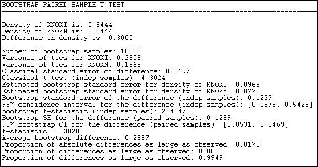
Results for both the standard approach and the bootstrap approach (this time, we ran 10,000 sub-samples) are reported in the output. The difference between means (or proportions, or densities) is .3000. The standard error of the difference by the classical method is .0697; the standard error by bootstrap estimate is .1237. The conventional approach greatly underestimates the true sampling variability, and gives a result that is too optimistic in rejecting the null hypothesis that the two densities are the same.
By the bootstrap method, we can see that there is a two-tailed probability of .0178. If we had a prior alternative hypothesis about the direction of the difference, we could use the one-tailed p level of .0052. So, we can conclude with great confidence that the density of information ties among organizations is greater than the density of monetary ties. That is, the observed difference would arise very rarely by chance in random samples drawn from these networks.
table of contentsIf there is a tie between two particular actors in one relation, is there likely to be a tie between them in another relation? If two actors have a strong tie of one type, are they also likely to have a strong tie of another?
When we have information about multiple relations among the same sets of actors, it is often of considerable interest whether the probability (or strength) of a tie of one type is related to the probability (or strength) of another. Consider the Knoke information and money ties. If organizations exchange information, this may create a sense of trust, making monetary exchange relations more likely; or, if they exchange money, this may facilitate more open communications. That is, we might hypothesize that the matrix of information relations would be positively correlated with the matrix of monetary relations - pairs that engage in one type of exchange are more likely to engage in the other. Alternatively, it might be that the relations are complementary: money flows in one direction, information in the other (a negative correlation). Or, it may be that the two relations have nothing to do with one another (no correlation).
Tools>Testing Hypotheses>Dyadic (QAP)>QAP Correlation calculates measures of nominal, ordinal, and interval association between the relations in two matrices, and uses quadratic assignment procedures to develop standard errors to test for the significance of association. Figure 18.8 shows the results for the correlation between the Knoke information and monetary exchange networks.
Figure 18.8. Association between Knoke information and Knoke monetary networks by QAP correlation

The first column shows the values of five alternative measures of association. The Pearson correlation is a standard measure when both matrices have valued relations measured at the interval level. Gamma would be a reasonable choice if one or both relations were measured on an ordinal scale. Simple matching and the Jaccard coefficient are reasonable measures when both relations are binary; the Hamming distance is a measure of dissimilarity or distance between the scores in one matrix and the scores in the other (it is the number of values that differ, element-wise, from one matrix to the other).
The third column (Avg) shows the average value of the measure of association across a large number of trials in which the rows and columns of the two matrices have been randomly permuted. That is, what would the correlation (or other measure) be, on the average, if we matched random actors? The idea of the "Quadratic Assignment Procedure" is to identify the value of the measure of association when their really isn't any systematic connection between the two relations. This value, as you can see, is not necessarily zero -- because different measures of association will have limited ranges of values based on the distributions of scores in the two matrices. We note, for example, that there is an observed simple matching of .456 (i.e. if there is a 1 in a cell in matrix one, there is a 45.6% chance that there will be a 1 in the corresponding cell of matrix two). This would seem to indicate association. But, because of the density of the two matrices, matching randomly re-arranged matrices will display an average matching of .475. So the observed measure differs hardly at all from a random result.
To test the hypothesis that there is association, we look at the proportion of random trials that would generate a coefficient as large as (or as small as, depending on the measure) the statistic actually observed. These figures are reported (from the random permutation trials) in the columns labeled "P(large)" and "P(small)." The appropriate one of these values to test the null hypothesis of no association is shown in the column "Signif."
table of contentsRather than correlating one relation with another, we may wish to predict one relation knowing the other. That is, rather than symmetric association between the relations, we may wish to examine asymmetric association. The standard tool for this question is linear regression, and the approach may be extended to using more than one independent variable.
Suppose, for example, that we wanted to see if we could predict which of the Knoke bureaucracies sent information to which others. We can treat the information exchange network as our "dependent" network (with N = 90).
We might hypothesize that the presence of a money tie from one organization to another would increase the likelihood of an information tie (of course, from the previous section, we know this isn't empirically supported!). Furthermore, we might hypothesize that institutionally similar organizations would be more likely to exchange information. So, we have created another 10 by 10 matrix, coding each element to be a "1" if both organizations in the dyad are governmental bodies, or both are non-governmental bodies, and "0" if they are of mixed types.
We can now perform a standard multiple regression analysis by regressing each element in the information network on its corresponding elements in the monetary network and the government institution network. To estimate standard errors for R-squared and for the regression coefficients, we can use quadratic assignment. We will run many trials with the rows and columns in the dependent matrix randomly shuffled, and recover the R-square and regression coefficients from these runs. These are then used to assemble empirical sampling distributions to estimate standard errors under the hypothesis of no association.
Version 6.81 of UCINET offers four alternative methods for Tools>Testing Hypotheses>Dyadic (QAP)>QAP Regression. Figure 18.9 shows the results of the "full partialling" method.
Figure 18.9. QAP regression of information ties on money ties and governmental status by full partialling method
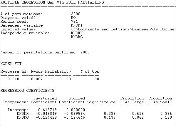
The descriptive statistics and measure of goodness of fit are standard multiple regression results -- except, of course, that we are looking at predicting relations between actors, not the attributes of actors.
The model R-square (.018) indicates that knowing whether one organization sends money to another, and whether the two organizations are institutionally similar reduces uncertainty in predicting an information tie by only about 2%. The significance level (by the QAP method) is .120. Usually, we would conclude that we cannot be sure the observed result is non-random.
Since the dependent matrix in this example is binary, the regression equation is interpretable as a linear probability model (one might want to consider logit or probit models -- but UCINET does not provide these). The intercept indicates that, if two organizations are not of the same institutional type, and one does not send money to the other, the probability that one sends information to the other is .61. If one organization does send money to the other, this reduces the probability of an information link by .046. If the two organizations are of the same institutional type, the probability of information sending is reduced by .124.
Using the QAP method, however, none of these effects are different from zero at conventional (e.g. p < .05) levels. The results are interesting - they suggest that monetary and informational linkages are, if anything, alternative rather than re-enforcing ties, and that institutionally similar organizations are less likely to communicate. But, we shouldn't take these apparent patterns seriously, because they could appear quite frequently simply by random permutation of the cases.
The tools in the this section are very useful for examining how multi-plex relations among a set of actors "go together." These tools can often be helpful additions to some of the tools for working with multi-plex data that we examined in chapter 16.
table of contentsIn the previous section we examined methods for testing differences and association among whole networks. That is, studying the macro-patterns of how an actor's position in one network might be associated with their position in another.
We are often interested in micro questions, as well. For example: does an actor's gender affect their between-ness centrality? This question relates an attribute (gender) to a measure of the actor's position in a network (between-ness centrality). We might be interested in the relationship between two (or more) aspects of actor's positions. For example: how much of the variation in actor's between-ness centrality can be explained by their out-degree and the number of cliques that they belong to? We might even be interested in the relationship between two individual attributes among a set of actors who are connected in a network. For example, in a school classroom, is there an association between actor's gender and their academic achievement?
In all of these cases we are focusing on variables that describe individual nodes. These variables may be either non-relational attributes (like gender), or variables that describe some aspect of an individual's relational position (like between-ness). In most cases, standard statistical tools for the analysis of variables can be applied to describe differences and associations.
But, standard statistical tools for the analysis of variables cannot be applied to inferential questions -- hypothesis or significance tests, because the individuals we are examining are not independent observations drawn at random from some large population. Instead of applying the normal formulas (i.e. those built into statistical software packages and discussed in most basic statistics texts), we need to use other methods to get more correct estimates of the reliability and stability of estimates (i.e. standard errors). The "boot-strapping" approach (estimating the variation of estimates of the parameter of interest from large numbers of random sub-samples of actors) can be applied in some cases; in other cases, the idea of random permutation can be applied to generate correct standard errors.
table of contentsSuppose we had the notion that private-for-profit organizations were less likely to actively engage in sharing information with others in their field than were government organizations. We would like to test this hypothesis by comparing the average out-degree of governmental and non-governmental actors in one organizational field.
Using the Knoke information exchange network, we've run Network>Centrality>Degree, and saved the results in the output file "FreemanDegree" as a UCINET dataset. We've also used Data>Spreadsheets>Matrix to create a UCINET attribute file "knokegovt" that has a single column dummy code (1 = governmental organization, 0 = non-governmental organization).
Let's perform a simple two-sample t-test to determine if the mean degree centrality of government organizations is lower than the mean degree centrality of non-government organizations. Figure 18.10 shows the dialog for Tools>Testing Hypotheses>Node-level>T-Test to set up this test.
Figure 18.10. Dialog for Tools>Testing Hypotheses>Node-level>T-Test

Since we are working with individual nodes as observations, the data are located in a column (or, sometimes, a row) of one or more files. Note how the file names (selected by browsing, or typed) and the columns within the file are entered in the dialog. The normed Freeman degree centrality measure happens to be located in the second column of its file; there is only one vector (column) in the file that we created to code government/non-government organizations.
For this test, we have selected the default of 10,000 trials to create the permutation-based sampling distribution of the difference between the two means. For each of these trials, the scores on normed Freeman degree centralization are randomly permuted (that is, randomly assigned to government or non-government, proportional to the number of each type.) The standard deviation of this distribution based on random trials becomes the estimated standard error for our test. Figure 18.11 shows the results.
Figure 18.11. Test for difference in mean normed degree centrality of Knoke government and non-government organizations
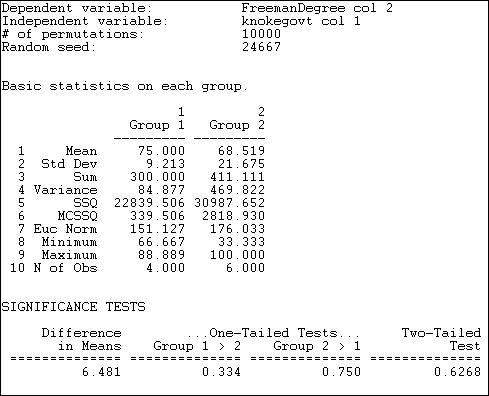
The output first reports basic descriptive statistics for each group. The group numbers are assigned according to the order of the cases in the file containing the independent variable. In our example, the first node was COUN, a government organization; so, government became "Group 1" and non-government became "Group 2."
We see that the average normed degree centrality of government organizations (75) is 6.481 units higher than the average normed degree centrality of non-governmental organizations (68.519). This would seem to support our hypothesis; but tests of statistical significance urge considerable caution. Differences as large as 6.481 in favor of government organizations happen 33.4% of the time in random trials -- so we would be taking an unacceptable risk of being wrong if we concluded that the data were consistent with our research hypothesis.
UCINET does not print the estimated standard error, or the values of the conventional two-group t-test.
table of contentsThe approach to estimating difference between the means of two groups discussed in the previous section can be extended to multiple groups with one-way analysis of variance (ANOVA). The procedure Tools>Testing Hypotheses>Node-level>Anova provides the regular OLS approach to estimating differences in group means. Because our observations are not independent, the procedure of estimating standard errors by random replications is also applied.
Suppose we divided the 23 large donors to California political campaigns into three groups, and have coded a single column vector in a UCINET attribute file. We've coded each donor as falling into one of three groups: "others," "capitalists," or "workers."
If we examine the network of connections among donors (defined by co-participating in the same campaigns), we anticipate that the worker's groups will display higher eigenvector centrality than donors in the other groups. That is, we anticipate that the "left" interest groups will display considerable interconnection, and -- on the average -- have members that are more connected to highly connected others than is true for the capitalist and other groups. We've calculated eigenvector centrality using Network>Centrality>Eigenvector, and stored the results in another UCINET attribute file.
The dialog for Tools>Testing Hypotheses>Node-level>Anova looks very much like Tools>Testing Hypotheses>Node-level>T-test, so we won't display it. The results of our analysis are shown as figure 18.12.
Figure 18.12. One-way ANOVA of eigenvector centrality of California political donors, with permutation-based standard errors and tests
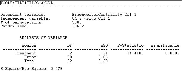
The mean eigenvector centrality of the eight "other" donors is .125. For the seven "capitalists" it is .106, and for the seven "workers" groups it is .323 (calculated elsewhere). The differences among these means is highly significant (F = 34.4 with 2 d.f. and p = .0002). The differences in group means account for 78% of the total variance in eigenvector centrality scores among the donors.
table of contentsWhere the attribute of actors that we are interested in explaining or predicting is measured at the interval level, and one or more of our predictors are also at the interval level, multiple linear regression is a common approach. Tools>Testing Hypotheses>Node-level>Regression will compute basic linear multiple regression statistics by OLS, and estimate standard errors and significance using the random permutations method for constructing sampling distributions of R-squared and slope coefficients.
Let's continue the example in the previous section. Our dependent attribute, as before, is the eigenvector centrality of the individual political donors. This time, we will use three independent vectors, which we have constructed using Data>Spreadsheets>Matrix, as shown in figure 18.13.
Figure 18.13. Construction of independent vectors for multiple linear regression
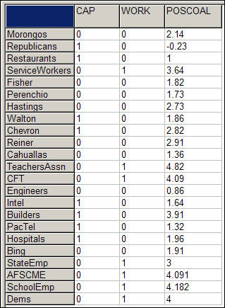
Two dummy variables have been constructed to indicate whether each donor is a member of the "capitalist" or the "worker" group. The omitted category ("other") will serve as the intercept/reference category. POSCOAL is the mean number of times that each donor participates on the same side of issues with other donors (a negative score indicates opposition to other donors).
Substantively, we are trying to find out whether the "workers" higher eigenvector centrality (observed in the section above) is simply a function of higher rates of participation in coalitions, or whether the workers have better connected allies -- independent of high participation.
Figure 18.14 shows the dialog to specify the dependent and the multiple independent vectors.
Figure 18.14. Dialog for Tools>Testing Hypotheses>Node-level>Regression for California donor's eigenvector centrality
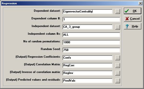
Note that all of the independent variables need to be entered into a single data set (with multiple columns). All of the basic regression statistics can be saved as output, for use in graphics or further analysis. Figure 18.15 shows the result of the multiple regression estimation.
Figure 18.15. Multiple regression of eigenvector centrality with permutation based significance tests
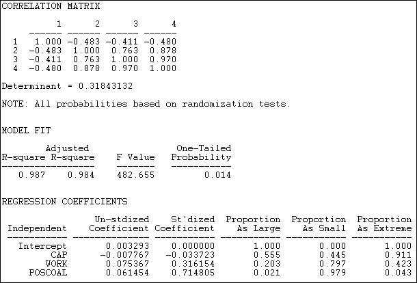
The correlation matrix shows a very high collinearity between being in the workers group (variable 3) and participation in coalitions (variable 4). This suggests that it may be difficult to separate effects of simple participation from those of being a workers interest group.
The R-squared is very high for this simple model (.987), and highly significant using permutation tests ( p = .014).
Controlling for total coalition participation, capitalist interests are likely to have slightly lower eigenvector centrality than others (-.0078), but this is not significant (p = .555). Workers groups do appear to have higher eigenvector centrality, even controlling for total coalition participation (.075), but this tendency may be a random result (a one-tailed significance is only p = .102). The higher the rate of participation in coalitions (POSCOAL), the greater the eigenvector centrality of actors (.0615, p = .021), regardless of which type of interest is being represented.
As before, the coefficients are generated by standard OLS linear modeling techniques, and are based on comparing scores on independent and dependent attributes of individual actors. What differs here is the recognition that the actors are not independent, so that estimation of standard errors by simulation, rather than by standard formula, is necessary.
The t-test, ANOVA, and regression approaches discussed in this section are all calculated at the micro, or individual actor level. The measures that are analyzed as independent and dependent may be either relational or non-relational. That is, we could be interested in predicting and testing hypotheses about actors non-relational attributes (e.g. their income) using a mix of relational (e.g. centrality) and non-relational (e.g. gender) attributes. We could be interested in predicting a relational attribute of actors (e.g. centrality) using a mix of relational and non-relational independent variables.
The examples illustrate how relational and non-relational attributes of actors can be analyzed using common statistical techniques. The key thing to remember, though, is that the observations are not independent (since all the actors are members of the same network). Because of this, direct estimation of the sampling distributions and resulting inferential statistics is needed -- standard, basic statistical software will not give correct answers.
table of contentsIn the previous section we looked at some tools for hypotheses about individual actors embedded in networks. Models like these are very useful for examining the relationships among relational and non-relational attributes of individuals.
One of the most distinctive ways in which statistical analysis has been applied to social network data is to focus on predicting the relations of actors, rather than their attributes. Rather than building a statistical model to predict each actor's out-degree, we could, instead, predict whether there was a tie from each actor to each other actor. Rather than explaining the variance in individual persons, we could focus on explaining variation in the relations.
In this final section, we will look at several statistical models that seek to predict the presence or absence (or strength) of a tie between two actors. Models like this are focusing directly on a very sociological question: what factors affect the likelihood that two individuals will have a relationship?
One obvious, but very important, predictor of whether two actors are likely to be connected is their similarity or closeness. In many sociological theories, two actors who share some attribute are predicted to be more likely to form social ties than two actors who do not. This "homophily" hypothesis is at the core of many theories of differentiation, solidarity, and conflict. Two actors who are closer to one in a network are often hypothesized to be more likely to form ties; two actors who share attributes are likely to be at closer distances to one another in networks.
Several of the models below explore homophily and closeness to predict whether actors have ties, or are close to one another. The last model that we will look at the "P1" model also seeks to explain relations. The P1 model tries to predict whether there exists no relation, an asymmetrical relation, or a reciprocated tie between pairs of actors. Rather than using attributes or closeness as predictors, however, the P1 model focuses on basic network properties of each actor and the network as a whole (in-degree, out-degree, global reciprocity). This type of model -- a probability model for the presence/absence of each possible relation in a graph as a function of network structures -- is one of the major continuing areas of development in social network methods.
table of contentsOne of the most commonplace sociological observations is that "birds of a feather flock together." The notion that similarity (or homophily) increases the probability of the formation of social ties is central to most sociological theories. The homophily hypothesis can be read to be making a prediction about social networks. It suggests that if two actors are similar in some way, it is more likely that there will be network ties between them. If we look at a social network that contains two types of actors, the density of ties ought to be greater within each group than between groups.
Tools>Testing Hypotheses>Mixed Dyadic/Nodal>Categorical Attributes>Joint-Count Provides a test that the density of ties within and between two groups differs from what we would expect if ties were distributed at random across all pairs of nodes.
The procedure takes a binary graph and a partition (that is, a vector that classifies each node as being in one group or the other), and permutes and blocks the data. If there was no association between sharing the same attribute (i.e. being in the same block) and the likelihood of a tie between two actors, we can predict the number of ties that ought to be present in each of the four blocks of the graph (that is: group 1 by group 1; group 1 by group 2; group 2 by group 1; and group 2 by group 2). These four "expected frequencies" can then be compared to the four "observed frequencies." The logic is exactly the same as the Pearson Chi-square test of independence -- we can generate a "test statistic" that shows how far the 2 by 2 table departs from "independence" or "no association."
To test the inferential significance of departures from randomness, however, we cannot rely on standard statistical tables. Instead, a large number of random graphs with the same overall density and the same sized partitions are calculated. The sampling distribution of differences between observed and expected for random graphs can then be calculated, and used to assess the likelihood that our observed graph could be a result of a random trial from a population where there was no association between group membership and the likelihood of a relation.
To illustrate, if two large political donors contributed on the same side of political campaigns (across 48 initiative campaigns), we code them "1" as having a tie or relation, otherwise, we code them zero. We've divided our large political donors in California initiative campaigns into two groups -- those that are affiliated with "workers" (e.g. unions, the Democratic party), and those that are not.
We would anticipate that two groups that represent workers interests would be more likely to share the tie of being in coalitions to support initiatives than would two groups drawn at random. Figure 18.16 shows the results of Tools>Testing Hypotheses>Mixed Dyadic/Nodal>Categorical Attributes>Joint-Count applied to this problem.
Figure 18.16. Test for two-group differences in tie density
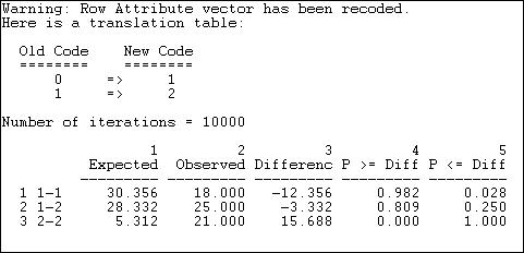
The partition vector (group identification variable) was originally coded as zero for non-worker donors and one for worker donors. These have been re-labeled in the output as one and two. We've used the default of 10,000 random graphs to generate the sampling distribution for group differences.
The first row, labeled "1-1" tells us that, under the null hypothesis that ties are randomly distributed across all actors (i.e. group makes no difference), we would expect 30.356 ties to be present in the non-worker to non-worker block. We actually observe 18 ties in this block, 12 fewer than would be expected. A negative difference this large occurred only 2.8% of the time in graphs where the ties were randomly distributed. It is clear that we have a deviation from randomness within the "non-worker" block. But the difference does not support homophily -- it suggest just the opposite; ties between actors who share the attribute of not representing workers are less likely than random, rather than more likely.
The second row, labeled "1-2" shows no significant difference between the number of ties observed between worker and non-worker groups and what would happen by chance under the null hypothesis of no effect of shared group membership on tie density.
The third row, labeled "2-2" A difference this large indicates that the observed count of ties among interest groups representing workers (21) is much greater than expected by chance (5.3).ould almost never be observed if the null hypothesis of no group effect on the probability of ties were true.
Perhaps our result does not support homophily theory because the group "non-worker" is not really as social group at all -- just a residual collection of diverse interests. Using Tools>Testing Hypotheses>Mixed Dyadic/Nodal>Categorical Attributes>Relational Contingency-Table Analysis we can expand the number of groups to provide a better test. This time, let's categorize the political donors as representing "others," "capitalists," or "workers." The results of this test are shown as figure 18.17.
Figure 18.17. Test for three-group differences in tie density
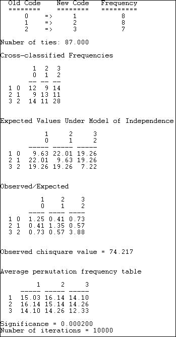
The "other" group has been re-labeled "1," the "capitalist" group re-labeled "2," and the "worker" group re-labeled "3." There are 87 total ties in the graph, with the observed frequencies shown ("Cross-classified Frequencies).
We can see that the the observed frequencies differ from the "Expected Values Under Model of Independence." The magnitudes of the over and under-representation are shown as "Observed/Expected." We note that all three diagonal cells (that is, ties within groups) now display homophily -- greater than random density.
A Pearson chi-square statistic is calculated (74.217). And, we are shown the average tie counts in each cell that occurred in the 10,000 random trials. Finally, we observe that p < .0002. That is, the deviation of ties from randomness is so great that it would happen only very rarely if the no-association model was true.
table of contentsThe result in the section above seems to support homophily (which we can see by looking at where the deviations from independence occur. The statistical test, though, is just a global test of difference from random distribution. The routine Tools>Testing Hypotheses>Mixed Dyadic/Nodal>Categorical Attributes>ANOVA Density Models provides specific tests of some quite specific homophily models.
The least-specific notion of how members of groups relate to members of other groups is simply that the groups differ. Members of one group may prefer to have ties only within their group; members of another group might prefer to have ties only outside of their group.
The Structural Blockmodel option of Tools>Testing Hypotheses>Mixed Dyadic/Nodal>Categorical Attributes>ANOVA Density Models provides a test that the patterns of within and between group ties differ across groups -- but does not specify in what way they may differ. Figure 18.18 shows the results of fitting this model to the data on strong coalition ties (sharing 4 or more campaigns) among "other," "capitalist," and "worker" interest groups.
Figure 18.18. Structural blockmodel of differences in group tie density
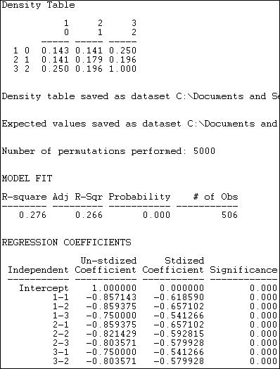
The observed density table is shown first. Members of the "other" group have a low probability of being tied to one another (.143) or to "capitalists" (.143), but somewhat stronger ties to "workers" (.250). Only the "workers" (category 2, row 3) show strong tendencies toward within-group ties.
Next, a regression model is fit to the data. The presence or absence of a tie between each pair of actors is regressed on a set of dummy variables that represent each of cells of the 3-by-3 table of blocks. In this regression, the last block (i.e. 3-3) is used as the reference category. In our example, the differences among blocks explain 27.6% of the variance in the pair-wise presence or absence of ties. The probability of a tie between two actors, both of whom are in the "workers" block (block 3) is 1.000. The probability in the block describing ties between "other" and "other" actors (block 1-1) is .857 less than this.
The statistical significance of this model cannot be properly assessed using standard formulas for independent observations. Instead, 5000 trials with random permutations of the presence and absence of ties between pairs of actors have been run, and estimated standard errors calculated from the resulting simulated sampling distribution.
A much more restricted notion of group differences is named the Constant Homophily model in Tools>Testing Hypotheses>Mixed Dyadic/Nodal>Categorical Attributes>ANOVA Density Models. This model proposes that all groups may have a preference for within-group ties, but that the strength of the preference is the same within all groups. The results of fitting this model to the data is shown in figure 18.19.
Figure 18.19. Constant Homophily blockmodel of differences in group tie density
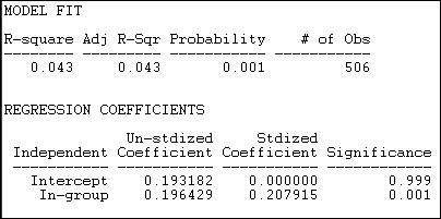
Given what we observed in looking directly at the block densities (shown in figure 18.18), it is not surprising that the constant homophily model does not fit these data well. We know that two of the groups ("others" and "capitalists") have no apparent tendency to homophily -- and that differs greatly from the "workers" group. The block model of group differences only accounts for 4.3% of the variance in pair-wise ties; however, permutation trials suggest that this is not a random result (p = .001).
This model only has two parameters, because the hypothesis is proposing a simple difference between the diagonal cells (the within group ties 1-1, 2-2, and 3-3) and all other cells. The hypothesis is that the densities within these two partitions are the same. We see that the estimated average tie density of pairs who are not in the same group is .193 -- there is a 19.3% chance that heterogeneous dyads will have a tie. If the members of the dyad are from the same group, the probability that they share a tie is .196 greater, or .389.
So, although the model of constant homophily does not predict individual's ties at all well, there is a notable overall homophily effect.
We noted that the strong tendency toward within-group ties appears to describe only the "workers" group. A third block model, labeled Variable Homophily by Tools>Testing Hypotheses>Mixed Dyadic/Nodal>Categorical Attributes>ANOVA Density Models tests the model that each diagonal cell (that is ties within group 1, within group 2, and within group 3) differ from all ties that are not within-group. Figure 18.20 displays the results.
Figure 18.20. Variable homophily blockmodel of differences in group tie density
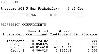
This model fits the data much better (R-square = .269, with p < .000) than the constant homophily model. It also fits the data nearly as well as the un-restricted structural block model (figure 18.18), but is simpler.
Here, the intercept is the probability that there well be a dyadic tie between any two members of different groups (.193). We see that the probability of within group ties among group 1 ("others") is actually .05 less than this (but not significantly different). Within group ties among capitalist interest groups (group 2) are very slightly less common (-.01) than heterogeneous group ties (again, not significant). Ties among interest groups representing workers (group 3) however, are dramatically more prevalent (.81) than ties within heterogeneous pairs.
In our example, we noted that one group seems to display in-group ties, and others do not. One way of thinking about this pattern is a "core-periphery" block model. There is a strong form, and a more relaxed form of the core-periphery structure.
The Core-periphery 1 model supposes that there is a highly organized core (many ties within the group), but that there are few other ties -- either among members of the periphery, or between members of the core and members of the periphery. Figure 18.21 shows the results of fitting this block model to the California donors data.
Figure 18.21. "Strong" core-periphery block model of California political donors
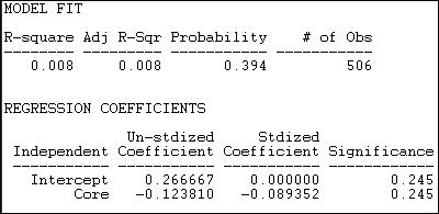
It's clear that this model does not do a good job of describing the pattern of within and between group ties. The R-square is very low (.008), and results this small would occur 39.4% of the time in trials from randomly permuted data. The (non-significant) regression coefficients show density (or the probability of a tie between two random actors) in the periphery as .27, and the density in the "Core" as .12 less than this. Since the "core" is, by definition, the maximally dense area, it appears that the output in version 6.8.5 may be mis-labeled.
Core-Periphery 2 offers a more relaxed block model in which the core remains densely tied within itself, but is allowed to have ties with the periphery. The periphery is, to the maximum degree possible, a set of cases with no ties within their group. Figure 18.22 shows the results of this model for the California political donors.
Figure 18.22. "Relaxed" core-periphery block model of California political donors
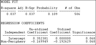
The fit of this model is better (R-square = .037) but still very poor. Results this strong would occur about 11% of the time in trials from randomly permuted data. The intercept density (which we interpret as the "non-periphery") is higher (about 35% of all ties are present), and the probability of a tie between two cases in the periphery is .17 lower.
table of contentsThe homophily hypothesis is often thought of in categorical terms: is there a tendency for actors who are of the same "type" to be adjacent (or close) to one another in the network?
This idea, though, can be generalized to continuous attributes: is there a tendency for actors who have more similar attributes to be located closer to one another in a network?
UCINET's Tools>Testing Hypotheses>Mixed Dyadic?Nodal>Continuous Attributes>Moran/Geary statistics provides two measures that address the question of the "autocorrelation" between actor's scores on interval-level measures of their attributes, and the network distance between them. The two measures (Moran's I and Geary's C) are adapted for social network analysis from their origins in geography, where they were developed to measure the extent to which the similarity of the geographical features of any two places was related to the spatial distance between them.
Let's suppose that we were interested in whether there was a tendency for political interest groups that were "close" to one another to spend similar amounts of money. We might suppose that interest groups that are frequent allies may also influence one another in terms of the levels of resources they contribute -- that a sort of norm of expected levels of contribution arises among frequent allies.
Using information about the contributions of very large donors (who gave over a total of $5,000,000) to at least four (of 48) ballot initiatives in California, we can illustrate the idea of network autocorrelation.
First, we create an attribute file that contains a column that has the attribute score of each node, in this case, the amount of total expenditures by the donors.
Second, we create a matrix data set that describes the "closeness" of each pair of actors. There are several alternative approaches here. One is to use an adjacency (binary) matrix. We will illustrate this by coding two donors as adjacent if they contributed funds on the same side of at least four campaigns (here, we've constructed adjacency from "affiliation" data; often we have a direct measure of adjacency, such as one donor naming another as an ally). We could also use a continuous measure of the strength of the tie between actors as a measure of "closeness." To illustrate this, we will use a scale of the similarity of the contribution profiles of donors that ranges from negative numbers (indicating that two donors gave money on opposite sides of initiatives) to positive numbers (indicating the number of times the donated on the same side of issues. One can easily imagine other approaches to indexing the network closeness of actors (e.g. 1/geodesic distance). Any "proximity" matrix that captures the pair-wise closeness of actors can be used (for some ideas, see Tools>Similarities and Tools>Dissimilarities and Distances).
Figures 18.23 and 18.24 display the results of Tools>Testing Hypotheses>Mixed Dyadic/Nodal>Continuous Attributes>Moran/Geary statistics where we have examined the autocorrelation of the levels of expenditures of actors using adjacency as our measure of network distance. Very simply: do actors who are adjacent in the network tend to give similar amounts of money? Two statistics and some related information are presented (the Moran statistic in figure 18.23, and the Geary statistic in figure 18.24.
Figure 18.23. Moran autocorrelation of expenditure levels by political donors with network adjacency

The Moran "I" statistic of autocorrelation (originally developed to measure spatial autocorrelation, but used here to measure network autocorrelation) ranges from -1.0 (perfect negative correlation) through 0 (no correlation) to +1.0 (perfect positive correlation). Here we see the value of -.119, indicating that there is a very modest tendency for actors who are adjacent to differ more in how much they contribute than two random actors. If anything, it appears that coalition members may vary more in their contribution levels than random actors -- another hypothesis bites the dust!
The Moran statistic (see any geo-statistics text, or do a Google search) is constructed very much like a regular correlation coefficient. It indexes the product of the differences between the scores of two actors and the mean, weighted by the actor's similarity - that is, a covariance weighted by the closeness of actors. This sum is taken in ratio to variance in the scores of all actors from the mean. The resulting measure, like the correlation coefficient, is a ratio of covariance to variance, and has a conventional interpretation.
Permutation trials are used to create a sampling distribution. Across many (in our example 1,000) trials, scores on the attribute (expenditure, in this case) are randomly assigned to actors, and the Moran statistic calculated. In these random trials, the average observed Moran statistic is -.043, with a standard deviation of .073. The difference between what we observe (-.119) and what is predicted by random association (-.043) is small relative to sampling variability. In fact, 17.4% of all samples from random data showed correlations at least this big -- far more than the conventional 5% acceptable error rate.
The Geary measure of correlation is calculated and interpreted somewhat differently. Results are shown in figure 18.24 for the association of expenditure levels by network adjacency.
Figure 18.24. Geary autocorrelation of expenditure levels by political donors with network adjacency
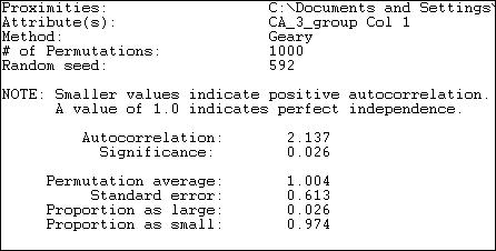
The Geary statistic has a value of 1.0 when there is no association. Values less than 1.0 indicate a positive association (somewhat confusingly), values greater than 1.0 indicate a negative association. Our calculated value of 2.137 indicates negative autocorrelation, just as the Moran statistic did. Unlike the Moran statistic though, the Geary statistic suggests that the difference of our result from the average of 1,000 random trials (1.004) is statistically significant (p = .026).
The Geary statistic is sometimes described in the geo-statistics literature as being more sensitive to "local" differences than to "global" differences. The Geary C statistic is constructed by examining the differences between the scores of each pair of actors, and weighting this by their adjacency. The Moran statistic is constructed by looking at differences between each actor's score and the mean, and weighting the cross-products. The difference in approach means that the Geary statistic is more focused on how different members of each pair are from each other - a "local" difference; the Moran statistic is focused more on how the similar or dissimilar each pair are to the overall average -- a "global" difference.
In data where the "landscape" of values displays a lot of variation, and non-normal distribution, the two measures are likely to give somewhat different impressions about the effects of network adjacency on similarity of attributes. As always, it's not that one is "right" and the other "wrong." It's always best to compute both, unless you have strong theoretical priors that suggest that one is superior for a particular purpose.
Figures 18.25 and 18.26 repeat the exercise above, but with one difference. In these two examples, we measure the closeness of two actors in the network on a continuous scale. Here, we've used the net number of campaigns on which each pair of actors were in the same coalition as a measure of closeness. Other measures, like geodesic distances might be more commonly used for true network data (rather than a network inferred from affiliation).
Figure 18.25. Moran autocorrelation of expenditure levels by political donors with network closeness
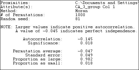
Using a continuous measure of network closeness (instead of adjacency) we might expect a stronger correlation. The Moran measure is now -.145 ( compared to -.119), and is significant at p = .018. There is a small, but significant tendency for actors who are "close" allies to give different amounts of money than two randomly chosen actors -- a negative network autocorrelation.
Figure 18.26. Geary autocorrelation of expenditure levels by political donors with network closeness

The Geary measure has become slightly smaller in size (1.836 versus 2.137) using a continuous measure of network distance. The result also indicates a negative autocorrelation, and one that would rarely occur by chance if there truly was no association between network distance and expenditure.
table of contentsThe approaches that we've been examining in this section look at the relationship between actor's attributes and their location in a network. Before closing our discussion of how statistical analysis has been applied to network data, we need to look at one approach that examines how ties between pairs of actors relate to particularly important relational attributes of the actors, and to a more global feature of the graph.
For any pair of actors in a directed graph, there are three possible relationships: no ties, an asymmetric tie, or a reciprocated tie. Network>P1 is a regression-like approach that seeks to predict the probability of each of these kinds of relationships for each pair of actors. This differs a bit from the approaches that we've examined so far which seek to predict either the presence/absence of a tie, or the strength of a tie.
The P1 model (and its newer successor the P* model), seek to predict the dyadic relations among actor pairs using key relational attributes of each actor, and of the graph as a whole. This differs from most of the approaches that we've seen above, which focus on actor's individual or relational attributes, but do not include overall structural features of the graph (at least not explicitly).
The P1 model consists of three prediction equations, designed to predict the probability of a mutual (i.e. reciprocated) relation (mij), an asymmetric relation (aij), or a null relation (nij) between actors. The equations, as stated by the authors of UCINET are:
mij = lambdaijexp(rho+2theta+alphai+alphaj+âi+âj)
aij = lambdaijexp(theta+alphai+betaj)
nij = lambdaij
The first equation says that the probability of a reciprocated tie between two
actors is a function of the out-degree (or "expansiveness") of each
actor: alphai and alphaj. It is also a
function of the overall density of the network (theta). It is also a
function of the global tendency in the whole network toward reciprocity (rho).
The equation also contains scaling constants for each actor in the pair (ai
and aj), as well as a global scaling parameter (lambda).
The second equation describes the probability that two actors will be connected with an asymmetric relation. This probability is a function of the overall network density (theta), and the propensity of one actor of the pair to send ties (expansiveness, or alpha), and the propensity of the other actor to receive ties ("attractiveness" or beta).
The probability of a null relation (no tie) between two actors is a "residual." That is, if ties are not mutual or asymmetric, they must be null. Only the scaling constant "lambda," and no causal parameters enter the third equation.
The core idea here is that we try to understand the relations between pairs of actors as functions of individual relational attributes (individual's tendencies to send ties, and to receive them) as well as key features of the graph in which the two actors are embedded (the overall density and overall tendency towards reciprocity). More recent versions of the model (P*, P2) include additional global features of the graph such as tendencies toward transitivity and the variance across actors in the propensity to send and receive ties.
Figure 18.27 shows the results of fitting the P1 model to the Knoke binary information network.
Figure 18.27. Results of P1 analysis of Knoke information network
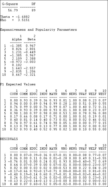
The technical aspects of the estimation of the P1 model are complicated, and maximum likelihood methods are used. A G-square (likelihood ratio chi-square) badness of fit statistic is provided, but has no direct interpretation or significance test.
Two descriptive parameters for global network properties are given:
Theta = -1.6882 refers to the effect of the global density of the network on the probability of reciprocated or asymmetric ties between pairs of actors.
Rho = 3.5151 refers to the effect of the overall amount of reciprocity in the global network on the probability of a reciprocated tie between any pair of actors.
Two descriptive parameters are given for each actor (these are estimated across all of the pair-wise relations of each actor):
Alpha ("expansiveness") refers to the effect of each actor's out-degree on the probability that they will have reciprocated or asymmetric ties with other actors. We see, for example, that the Mayor (actor 5) is a relatively "expansive" actor.
Beta ("attractiveness") refers to the effect of each actor's in-degree on the probability that they will have a reciprocated or asymmetric relation with other actors. We see here, for example, that the welfare rights organization (actor 6) is very likely to be shunned.
Using the equations, it is possible to predict the probability of each directed tie based on the model's parameters. These are shown as the "P1 expected values." For example, the model predicts a 93% chance of a tie from actor 1 to actor 2.
The final panel of the output shows the difference between the ties that actually exist, and the predictions of the model. The model predicts the tie from actor 1 to actor 2 quite well (residual = .07), but it does a poor job of predicting the relation from actor 1 to actor 9 (residual = .77).
The residuals important because they suggest places where other features of the graph or individuals may be relevant to understanding particular dyads, or where the ties between two actors is well accounted for by basic "demographics" of the network. Which actors are likely to have ties that are not predicted by the parameters of the model can also be shown in a dendogram, as in figure 18.28.
Figure 18.28. Diagram of P1 clustering of Knoke information network
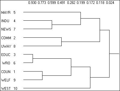
Here we see that, for example, that actors 3 and 6 are much more likely to have ties than the P1 model predicts.
table of contentsIn this chapter we've taken a look at some of the most basic and common approaches to applying statistical analysis to the attributes of actors embedded in networks, the relations among these actors, and the similarities between multiple relational networks connecting the same actors. We've covered a lot of ground. But, there is still a good bit more, as the application of statistical modeling to network data is one of the "leading edges" of the field of social (and other) network analyses.
There are two main reasons for the interest in applying statistics to what was, originally, deterministic graph theory from mathematics. First, for very large networks, methods for finding and describing the distributions of network features provide important tools for understanding the likely patterns of behavior of the whole network and the actors embedded in it. Second, we have increasingly come to realize that the relations we see among actors in a network at a point in time are best seen as probabilistic ("stochastic") outcomes of underlying processes of evolution of networks, and probabilistic actions of actors embedded in those networks. Statistical methods provide ways of dealing with description and hypothesis testing that take this uncertainty into account.
We've reviewed methods for examining relations between two (or more) graphs involving the same actors. These tools are particularly useful for trying to understand multi-plex relations, and for testing hypotheses about how the pattern of relations in one whole network relate to the pattern of relations in another.
We've also looked at tools that deal individual nodes. These tools allow us to examine hypotheses about the relational and non-relational attributes of actors, and to draw correct inferences about relations between variables when the observations (actors) are not independent.
And, we've taken a look at a variety of approaches that relate attributes of actors to their positions in networks. Much of the focus here is on how attributes may pattern relations (e.g. homophily), or how network closeness of distance may affect similarity of attributes (or vice versa).
Taken together, the marriage of statistics and mathematics in social network analysis has already produced some very useful ways of looking at patterns of social relations. It is likely that this interface will be one of the areas of most rapid development in the field of social network methods in the coming years.