17. Two-mode networks
For a classic study of the American south (Deep South, University of Chicago Press, 1941), Davis and his colleagues collected data on which of 18 women were present at each of the 14 events of the "social season" in a community. By examining patterns of which women are present (or absent) at which events, it is possible to infer an underlying pattern of social ties, factions, and groupings among the women. At the same time, by examining which women were present at the 14 events, it is possible to infer underlying patterns in the similarity of the events.
The Davis study is an example of what Ron Breiger (1974) called "The duality of persons and groups." Breiger is calling attention to the dual focus of social network analysis on how individuals, by their agency, create social structures while, at the same time, social structures develop an institutionalized reality that constrains and shapes the behavior of the individuals embedded in them.
The data used for social network analysis, most commonly, measure relations at the micro level, and use analysis techniques to infer the presence of social structure at the macro level. For example, we examine the ties of individuals (micro) for patterns that allow us to infer macro structure (i.e. cliques).
The Davis data is a bit different. It describes ties between two sets of nodes at two different levels of analysis. The ties that Davis identifies are between actors (the women) and events (the parties of the social season). Data like these involve two levels of analysis (or two "modes"). Often, such data are termed "affiliation" data because they describe which actors are affiliated (present, or members of) which macro structures.
Two-mode data offer some very interesting analytic possibilities for gaining greater understanding of "macro-micro" relations. In the Davis data, for example, we can see how the choices of the individual women "make" the meaning of the parties by choosing to attend or not. We can also see how the parties, as macro structures may affect the choices of the individual women.
With a little creativity, you can begin to see examples of these kinds of two-mode, or macro-micro social structures everywhere. The social world is one of "nesting" in which individuals (and larger structures) are embedded in larger structures (and larger structures are embedded in still larger ones). Indeed, the analysis of the tension between "structure and agency" or "macro and micro" is one of the core themes in sociological theory and analysis.
In this chapter we will take a look at some of the tools that have been applied (and, in some cases, developed) by social network analysts for examining two-mode data. We begin with a discussion of data structures, proceed to visualization, and then turn our attention to techniques for identifying quantitative and qualitative patterns in two-mode data.
For most of the examples in this chapter we will use a new 2-mode data set from a problem that I happen to be working on in parallel with this chapter. The data describe the contributions of a small number of large donors (those who gave a total of at least $1,000,000) to campaigns supporting and opposing ballot initiatives in California during the period 2000 to 2004. We've included 44 of the initiatives. The data set has two modes: donors and initiatives.
We will use two different forms of the data - one valued and one binary. The valued data describe the relations between donors and initiatives using a simple ordinal scale. An actors is coded as -1 if they gave a contribution opposing a particular initiative, 0 if they did not contribute, and +1 if they contributed in support of the initiative. The binary data describe whether a donor did (+1) or did not (0) contribute in the campaign on each initiative.
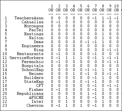
table of contentsThe most common way of storing 2-mode data is a rectangular data matrix of actors (rows) by events (columns). Figure 17.1 shows a portion of the valued data set we will use here (Data>Display).
Figure 17.1. Rectangular data array of California political donations data

The California Teachers Association, for example, gave donations in opposition to the 7th, 9th, and 10th ballot initiative, and a donation supporting the 8th.
A very common and very useful approach to two-mode data is to convert it into two one-mode data sets, and examine relations within each mode separately. For example, we could create a data set of actor-by-actor ties, measuring the strength of the tie between each pair of actors by the number of times that they contributed on the same side of initiatives, summed across the 40-some initiatives. We could also create a one-mode data set of initiative-by-initiative ties, coding the strength of the relation as the number of donors that each pair of initiatives had in common. The Data>Affiliations tool can be used to create one-mode data sets from a two-mode rectangular data array. Figure 17.2 displays a typical dialog box.
Figure 17.2. Dialog of Data>Affiliations to create actor-by-actor relations of California donors
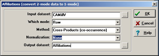
There are several choices here.
We have selected the row mode (actors) for this example. To create an initiative-by-initiative one-mode data set, we would have selected column.
There are two alternative methods:
The cross-product method takes each entry of the row for actor A, and multiplies it times the same entry for actor B, and then sums the result. Usually, this method is used for binary data because the result is a count of co-occurrence. With binary data, each product is 1 only if both actors were "present" at the event, and the sum across events yields the number of events in common - a valued measure of strength.
Our example is a little more complicated because we've applied the cross-product method to valued data. Here, if neither actor donated to an initiative (0 * 0 = 0), or if one donated and the other did not (0 * -1 or 0 * +1 = 0), there is no tie. If both donated in the same direction (-1 * -1 = 1 or +1 * +1 = 1) there is a positive tie. If both donated, but in opposite directions (+1 * -1 = -1) there is a negative tie. The sum of the cross-products is a valued count of the preponderance of positive or negative ties.
The minimums method examines the entries for the two actors at each event, and selects the minimum value. For binary data, the result is the same as the cross-product method (if both, or either actor is zero, the minimum is zero; only if both are one is the minimum one). For valued data, the minimums method is essentially saying: the tie between the two actors is equal to the weaker of the ties of the two actors to the event. This approach is commonly used when the original data are measured as valued.
Figure 17.3 shows the result of applying the cross-products method to our valued data.
Figure 17.3. Actor-by-actor tie strengths (Figure 17.2)
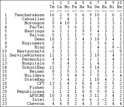
The teachers association participated in 16 campaigns (the cross-product of the row with itself counts the number of events). The association took the same position on issues as the Democratic party (actor 7) ten more times than taking opposite (or no) position. The restaurant association (node 10) took an opposite position to Mr. Bing (node 9) more frequently than supporting (or no) position. Using this algorithm, we've captured much, but not all of the information in the original data. A score of -1, for example, could be the result of two actors taking opposite positions on a single issue; or, it could mean that the two actors both took positions on several issues -- and, in sum, they disagreed one more time than they agreed.
The resulting one-mode matrices of actors-by-actors and events-by-events are now valued matrices indicating the strength of the tie based on co-occurrence. Any of the methods for one-mode analysis can now be applied to these matrices to study either micro structure or macro structure.
Two-mode data are sometimes stored in a second way, called the "bipartite" matrix. A bipartite matrix is formed by adding the rows as additional columns, and columns as additional rows. For example, a bipartite matrix of our donors data would have 68 rows (the 23 actors followed by the 45 initiatives) by 68 columns (the 23 actors followed by the 45 initiatives). The two actor-by-event blocks of the matrix are identical to the original matrix; the two new blocks (actors by actors and events by events) are usually coded as zeros. The Transform>Bipartite tool converts two-mode rectangular matrices to two-mode bipartite matrices. Figure 17.4 shows a typical dialog.
Figure 17.4 Dialog of Transform>Bipartite for California political donations data

The value to fill within-mode ties usually zero, so that actors are connected only by co-presence at events, and events are connected only by having actors in common.
Once data have been put in the form of a square bipartite matrix, many of the algorithms discussed elsewhere in this text for one-mode data can be applied. Considerable caution is needed in interpretation, because the network that is being analyzed is a very unusual one in which the relations are ties between nodes at different levels of analysis. In a sense, actors and events are being treated as social objects at a single level of analysis, and properties like centrality and connection can be explored. This type of analysis is relatively rare, but does have some interesting creative possibilities.
More commonly, we seek to keep the actors and events "separate" but "connected" and to seek patterns in how actors tie events together, and how events tie actors together. We will examine a few techniques for this task, below. A good first step in any network analysis though is to visualize the data.
table of contentsThere are no new technical issues in using graphs to visualize 2-mode data. Both actors and events are treated as nodes, and lines are used to show the connections of actors to events (there will be no lines from actors to actors directly, or from events to events).
In UCINET, the tool NetDraw>File>Open>UCINET dataset>2-Mode Network produces a useful graph for small networks. Figure 17.5 shows one rendering of the California donors data in its valued form.
Figure 17.5. Two-mode valued network of California donors and initiatives
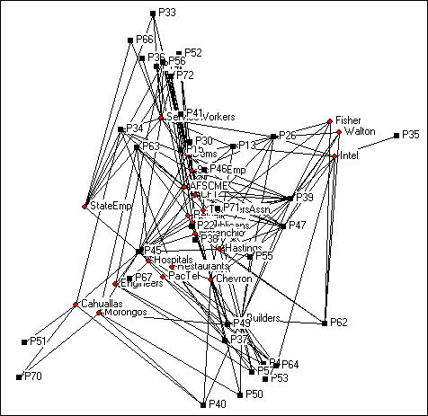
Since the graphic has 68 nodes (actors plus initiatives) it is a bit cluttered. We've deleted isolates (initiatives that don't have donors in common and donors that don't have initiatives in common), located the points in space using Gower MDS, resized the nodes and node labels, and eliminated the arrow heads.
We can get some insights from this kind of visualization of a two-mode network (particularly when some kind of scaling method is used to locate the points in space). Actors that are close together (e.g. the Cahualla and Morongo Indians in the lower left corner) are connected because they have similar profiles of events. In this particular case, the two tribes were jointly involved in initiatives about gambling (P70) and environment (P40). Similarly, certain of the ballot propositions are "similar" in that they have donors in common. And, particular donors are located in the same parts of the space as certain initiatives -- defining which issues (events) tend to go along with which actors.
It is exactly this kind of "going together-ness" or "correspondence" of the locations of actors and events that the numeric methods discussed below are intended to index. That is, the numeric methods are efforts to capture the clustering of actors brought together by events; events brought together by the co-presence of actors; and the resulting "bundles" of actors/events.
table of contentsWhen we are working with a large number of variables that describe aspects of some phenomenon (e.g. items on a test as multiple measures of the underlying trait of "mastery of subject matter"), we often focus our attention on what these multiple measures have "in common." Using information about the co-variation among the multiple measures, we can infer an underlying dimension or factor; once we've done that, we can locate our observations along this dimension. The approach of locating, or scoring, individual cases in terms of their scores on factors of the common variance among multiple indicators is the goal of factor and components analysis (and some other less common scaling techniques).
If we think about our two-mode problem, we could apply this "scaling" logic to either actors or to events. That is, we could "scale" or index the similarity of the actors in terms of their participation in events - but weight the events according to common variance among them. Similarly, we could "scale" the events in terms of the patterns of co-participation of actors -- but weight the actors according to their frequency of co-occurrence. Techniques like Tools>MDS and factor or principal components analysis could be used to "scale" either actors or events.
It is also possible to apply these kinds of scaling logics to actor-by-event data. UCINET includes two closely-related factor analytic techniques (Tools>2-Mode Scaling>SVD and Tools>2-Mode Scaling Factor Analysis) that examine the variance in common among both actors and events simultaneously. UCINET also includes Tools>2-Mode Scaling>Correspondence which applies the same logic to binary data. Once the underlying dimensions of the joint variance have been identified, we can then "map" both actors and events into the same "space." This allows us to see which actors are similar in terms of their participation in events (that have been weighted to reflect common patterns), which events are similar in terms of what actors participate in them (weighted to reflect common patterns), and which actors and events are located "close" to one another.
It is sometimes possible to interpret the underlying factors or dimensions to gain insights into why actors and events go together in the ways that they do. More generally, clusters of actors and events that are similarly located may form meaningful "types" or "domains" of social action.
Below, we will very briefly apply these tools to the data on large donors to California initiatives in the 2000-2004 period. Our goal is to illustrate the logic of 2-mode scaling. The discussion here is very short on technical treatments of the (important) differences among the techniques.
table of contentsSingular value decomposition (SVD) is one method of identifying the factors underlying two-mode (valued) data. The method of extracting factors (singular values) differs somewhat from conventional factor and components analysis, so it is a good idea to examine both SVD and 2-mode factoring results.
To illustrate SVD, we have input a matrix of 23 major donors (those who gave a combined total of more than $1,000,000 to five or more campaigns) by 44 California ballot initiatives. Each actor is scored as -1 if they contributed in opposition to the initiative, +1 if they contributed in favor of the initiative, or 0 if they did not contribute. The resulting matrix is valued data that can be examined with SVD and factor analysis; however, the low number of contributors to many initiatives, and the very restricted variance of the scale are not ideal.
Figure 17.6 shows the "singular values" extracted from the rectangular donor-by-initiative matrix using Tools>2-Mode Scaling>SVD.
Figure 17.6. Two-mode scaling of California donors and initiatives by Single Value Decomposition: Singular values
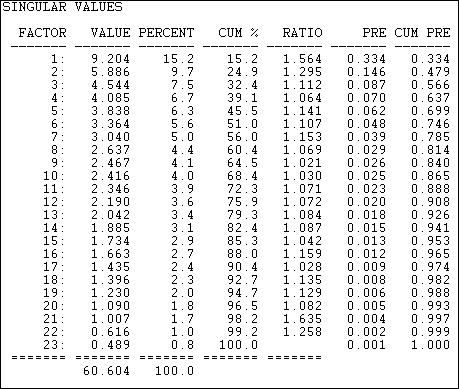
The "singular values" are analogous to "eigenvalues" in the more common factor and components scaling techniques. The result here shows that the joint "space" of the variance among donors and initiatives is not well captured by an simple characterization. If we could easily make sense of the patterns with ideas like "left/right" and "financial/moral" as underlying dimensions, there would be only a few singular values that explained substantial portions of the joint variance. This result tells us that the ways that actors and events "go together" is not clean, simple, and easy -- in this case.
With this important caveat in mind, we can examine how the events and donors are "scaled" or located on the underlying dimensions. First, the ballot initiatives. Figure 17.7 shows the location, or scale scores of each of the ballot proposition on the first six underlying dimensions of this highly multi-dimensional space.
Figure 17.7. SVD of California donors and initiatives: Scaling of initiatives
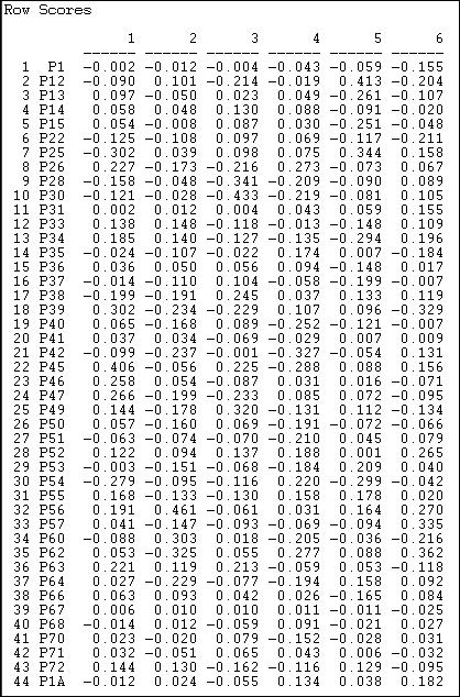
It turns out that the first dimension tends to locate initiatives supporting public expenditure for education and social welfare toward one pole, and initiatives supporting limitation of legislative power toward the other -- though interpretations like this are entirely subjective. The second and higher dimensions seem to suggest that initiatives can also be seen as differing from one another in other ways.
At the same time, the results let us locate or scale the donors along the same underlying dimensions. These loadings are shown in Figure 17.8.
Figure 17.8. SVD of California donors and initiatives: Scaling of donors
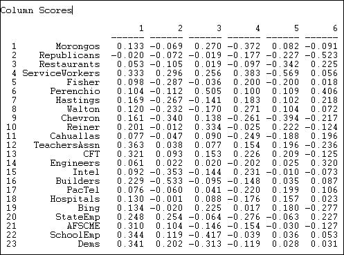
Toward the positive end of dimension one (which we earlier interpreted as favoring public expenditure) we find the Democratic party, public employees and teachers unions; at the opposite pole, we find Republicans and some business and professional groups.
It is often useful to visualize the locations of the actors and events in a scatterplot defined by scale scores on the various dimensions. The map in Figure 17.9 shows the results for the first two dimensions of this space.
Figure 17.9. SVD of California donors and initiatives: Two-dimensional map
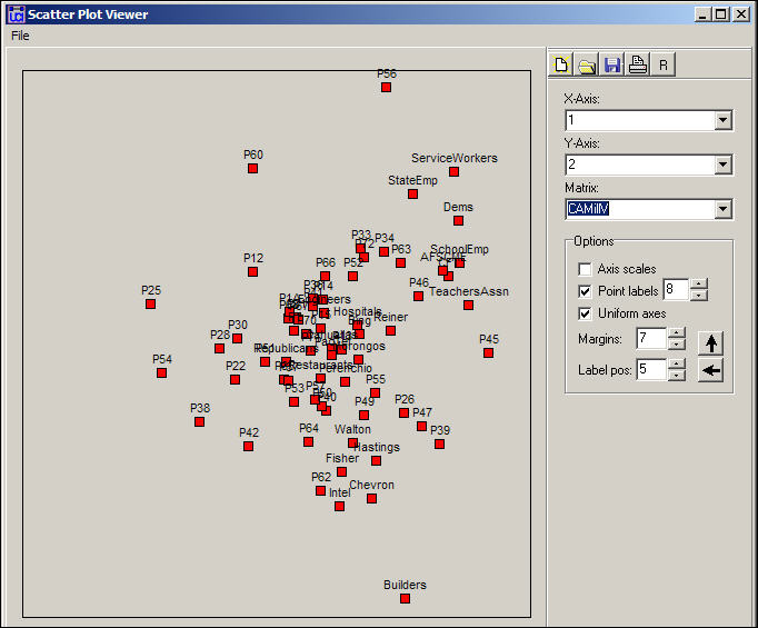
We note that the first dimension (left-right in the figure) seems to have its poles "anchored" by differences among the initiatives; the second dimension (top-bottom) seems to be defined more by differences among groups (with the exception of proposition 56). The result does not cleanly and clearly locate particular events and particular actors along strong linear dimensions. It does, however, produce some interesting clusters that show groups of actors along with the issues that are central to their patterns of participation. The Democrats and unions cluster (upper right) along with a number of particular propositions in which they were highly active (e.g. 46, 63). Corporate, building, and venture capitalist cluster (more loosely) in the lower right, along with core issues that formed their primary agenda in the initiative process (e.g. prop. 62).
table of contentsFactor analysis provides an alternative method to SVD to the same goals: identifying underlying dimensions of the joint space of actor-by-event variance, and locating or scaling actors and events in that space. The method used by factor analysis to identify the dimensions differs from SVD. Figure 17.10 shows the eigenvalues (by principle components) calculated by Tools>2-Mode Scaling>Factor Analysis.
Figure 17.10 Eigenvalues of two-mode factoring of California donors and initiatives
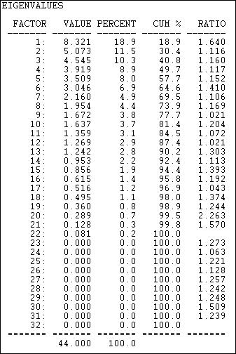
This solution, although different from SVD, also suggests considerable dimensional complexity in the joint variance of actors and events. That is, simple characterizations of the underlying dimensions (e.g. "left/right") do not provide very accurate predictions about the locations of individual actors or events. The factor analysis method does produce somewhat lower complexity than SVD.
With the caveat of pretty poor fit of a low-dimensional solution in mind, let's examine the scaling of actors on the first three factors (figure 17.11).
Figure 17.11. Loadings of donors
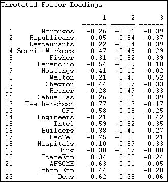
The first factor, by this method, produces a similar pattern to SVD. At one pole are Democrats and unions, at the other lie many capitalist groups. There are, however, some notable differences (e.g. AFSCME). Figure 17.12 shows the loadings of the events.
Figure 17.12. Loadings of events
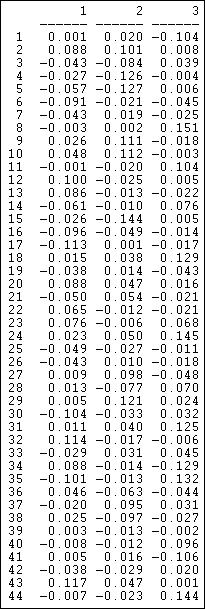
The patterns here also have some similarity to the SVD results, but do differ considerably in the specifics. To visualize the patterns, the loadings of actors and events on the dimensions could be extracted from output data files, and graphed using a scatterplot.
table of contentsFor binary data, the use of factor analysis and SVD is not recommended. Factoring methods operate on the variance/covariance or correlation matrices among actors and events. When the connections of actors to events is measured at the binary level (which is very often the case in network analysis) correlations may seriously understate covariance and make patterns difficult to discern.
As an alternative for binary actor-by-event scaling, the method of correspondence analysis (Tools>2-Mode Scaling>Correspondence) can be used. Correspondence analysis (rather like Latent Class Analysis) operates on multi-variate binary cross-tabulations, and its distributional assumptions are better suited to binary data.
To illustrate the application of correspondence analysis, we've dichotomized the political donor and initiatives data by assigning a value of 1 if an actor gave a donation either in favor or against an initiative, and assigning a zero if they did not participate in the campaign on a particular initiative. If we wanted our analysis to pay attention to partisanship, rather than simple participation, we could have created two data sets - one based on opposition or not, one based on support or not - and done two separate correspondence analyses.
Figure 17.13 shows the location of events (initiatives) along three dimensions of the joint actor-event space identified by the correspondence analysis method.
Figure 17.13. Event coordinates for co-participation of donors in California initiative campaigns
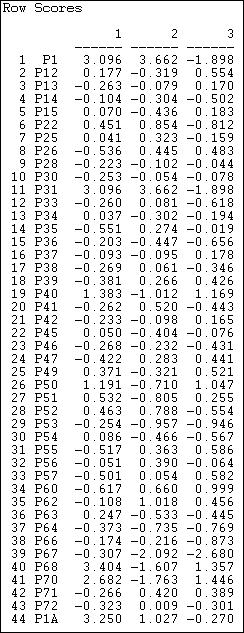
Since these data do not reflect partisanship, only participation, we would not expect the findings to parallel those discussed in the sections above. And, they don't. We do see, however, that this method also can be used to locate the initiatives along multiple underlying dimensions that capture variance in both actors and events. Figure 17.14 shows the scaling of the actors.
Figure 17.14. Actor coordinates for co-participation of donors in California initiative campaigns
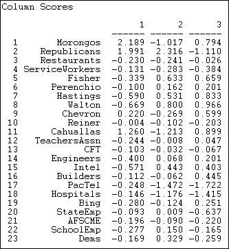
The first dimension here does have some similarity to the Democrat/union versus capitalist poles. Here, however, this difference means that the two groupings tend to participate in different groups of initiatives, rather than confronting one another in the same campaigns.
Visualization is often the best approach to finding meaningful patterns (in the absence of a strong theory). Figure 17.15 show the plot of the actors and events in the first two dimensions of the joint correspondence analysis space.
Figure 17.15. Correspondence analysis two-dimensional map
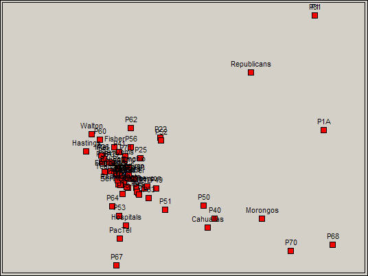
The lower right quadrant here contains a meaningful cluster of actors and events, and illustrates how the results of correspondence analysis can be interpreted. In the lower right we have some propositions regarding Indian casino gambling (68 and 70) and two propositions regarding ecological/conservation issues (40 and 50). Two of the major Native American Nations (the Cahualla and Morongo band of Mission Indians) are mapped together. The result is showing that there is a cluster of issues that "co-occur" with a cluster of donors - actors defining events, and events defining actors.
table of contentsOften all that we know about actors and events is simple co-presence. That is, either an actor was, or wasn't present, and our incidence matrix is binary. In cases like this, the scaling methods discussed above can be applied, but one should be very cautious about the results. This is because the various dimensional methods operate on similarity/distance matrices, and measures like correlations (as used in two-mode factor analysis) can be misleading with binary data. Even correspondence analysis, which is more friendly to binary data, can be troublesome when data are sparse.
An alternative approach is block modeling. Block modeling works directly on the binary incidence matrix by trying to permute rows and columns to fit, as closely as possible, idealized images. This approach doesn't involve any of the distributional assumptions that are made in scaling analysis.
In principle, one could fit any sort of block model to actor-by-event incidence data. We will examine two models that ask meaningful (alternative) questions about the patterns of linkage between actors and events. Both of these models can be directly calculated in UCINET. Alternative block models, of course, could be fit to incidence data using more general block-modeling algorithms.
table of contentsThe core-periphery structure is an ideal typical pattern that divides both the rows and the columns into two classes. One of the blocks on the main diagonal (the core) is a high-density block; the other block on the main diagonal (the periphery) is a low-density block. The core-periphery model is indifferent to the density of ties in the off-diagonal blocks.
When we apply the core-periphery model to actor-by-actor data (see Network>Core/Periphery), the model seeks to identify a set of actors who have high density of ties among themselves (the core) by sharing many events in common, and another set of actors who have very low density of ties among themselves (the periphery) by having few events in common. Actors in the core are able to coordinate their actions, those in the periphery are not. As a consequence, actors in the core are at a structural advantage in exchange relations with actors in the periphery.
When we apply the core-periphery model to actor-by-event data (Network>2-Mode>Categorical Core/Periphery) we are seeking the same idealized "image" of a high and a low density block along the main diagonal. But, now the meaning is rather different.
The "core" consists of a partition of actors that are closely connected to each of the events in an event partition; and simultaneously a partition of events that are closely connected to the actors in the core partition. So, the "core" is a cluster of frequently co-occurring actors and events. The "periphery" consists of a partition of actors who are not co-incident to the same events; and a partition of events that are disjoint because they have no actors in common.
Network>2-Mode>Categorical Core/Periphery uses numerical methods to search for the partition of actors and of events that comes as close as possible to the idealized image. Figure 17.16 shows a portion of the results of applying this method to participation (not partisanship) in the California donors and initiatives data.
Figure 17.16 Categorical core-periphery model of California $1M donors and ballot initiatives (truncated)
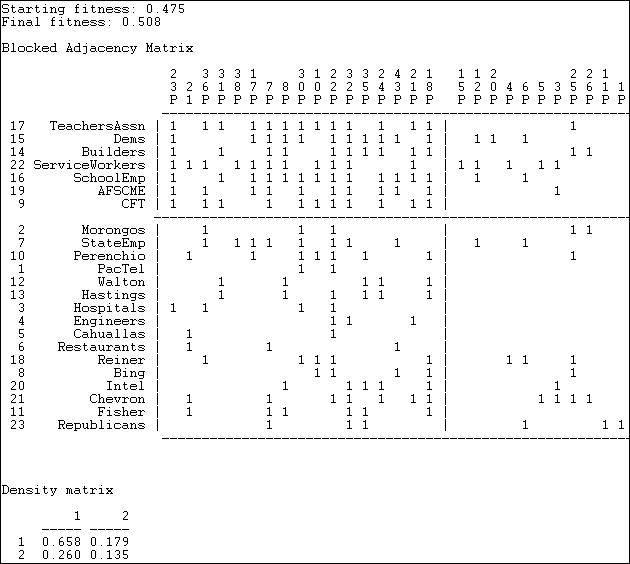
The numerical search method used by Network>2-Mode>Categorical Core/Periphery is a genetic algorithm, and the measure of goodness of fit is stated in terms of a "fitness" score (0 means bad fit, 1 means excellent fit). You can also judge the goodness of the result by examining the density matrix at the end of the output. If the block model was completely successful, the 1,1, block should have a density of one, and the 2, 2 block should have a density of zero. While far from perfect, the model here is good enough to be taken seriously.
The blocked matrix shows a "core" composed of the Democratic Party, a number of major unions, and the building industry association who are all very likely to participate in a considerable number of initiatives (proposition 23 through proposition 18). The remainder of the actors are grouped into the periphery as both participating less frequently, and having few issues in common. A considerable number of issues are also grouped as "peripheral" in the sense that they attract few donors, and these donors have little in common. We also see (upper right) that core actors do participate to some degree (.179) in peripheral issues. In the lower left, we see that peripheral actors participate somewhat more heavily (.260) in core issues.
table of contentsAn alternative block model is that of "factions." Factions are groupings that have high density within the group, and low density of ties between groups. Networks>Subgroups>Factions fits this block model to one-mode data (for any user-specified number of factions). Network>2-Mode>2-Mode Factions fits the same type of model to two-mode data (but for only two factions).
When we apply the factions model to one-mode actor data, we are trying to identify two clusters of actors who are closely tied to one another by attending all of the same events, but very loosely connected to members of other factions and the events that tie them together. If we were to apply the idea of factions to events in a one-mode analysis, we would be seeking to identify events that were closely tied by having exactly the same participants.
Network>2-Mode>2-Mode Factions applies the same approach to the rectangular actor-by-event matrix. In doing this, we are trying to locate joint groupings of actors and events that are as mutually exclusive as possible. In principle, there could be more than two such factions. Figure 17.17 shows the results of the two-mode factions block model to the participation of top donors in political initiatives.
Figure 17.17. Two mode factions model of California $1M donors and ballot initiatives (truncated)
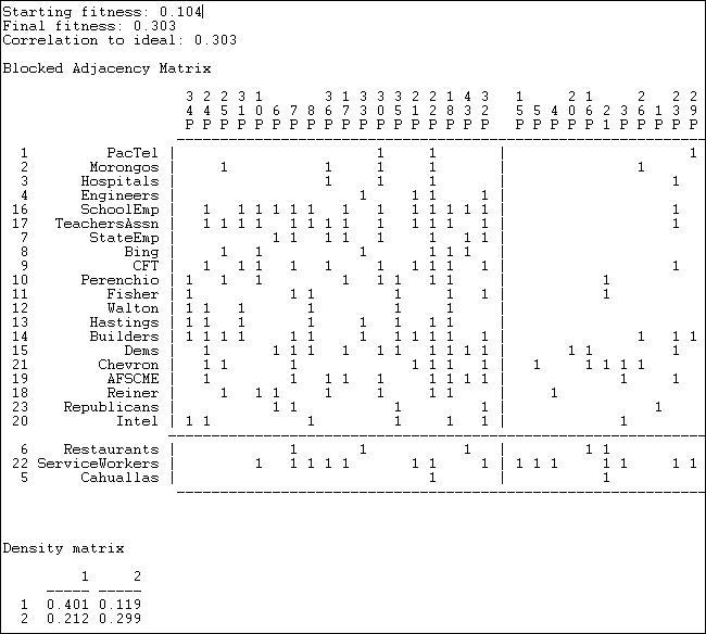
Two measures of goodness-of-fit are available. First we have our "fitness" score, which is the correlation between the observed scores (0 or 1) and the scores that "should" be present in each block. The densities in the blocks also informs us about goodness of fit. For a factions analysis, an ideal pattern would be dense 1-blocks along the diagonal (many ties within groups) and zero-blocks off the diagonal (ties between groups).
The fit of the two factions model is not as impressive as the fit of the core-periphery model. This suggests that an "image" of California politics as one of two separate and largely disjoint issue-actor spaces is not as useful as an image of a high intensity core of actors and issues coupled with an otherwise disjoint set of issues and participants.
The blocking itself also is not very appealing, placing most of the actors in one faction (with modest density of .401). The second faction is small, and has a density (.299) that is not very different from the off-diagonal blocks. As before, the blocking of actors by events is grouping together sets of actors and events that define one another.
table of contentsOne of the major continuing themes of social network analysis is the way in which individual actors "make" larger social structures by their patterns of interaction while, at the same time, institutional patterns shape the choices made by the individuals who are embedded within structures.
Two-mode data (often referred to as "actor-by-event" or "affiliation" in social network analysis) offer some interesting possibilities for gaining insights into macro-micro or agent-structure relations. With two-mode data, we can examine how macro-structures (events) pattern the interactions among agents (or not); we can also examine how the actors define and create macro structures by their patterns of affiliation with them. In addition, we can attempt to describe patterns of relations between actors and structures simultaneously.
In this chapter we briefly examined some of the typical ways in which two-mode data arise in social network analysis, and the data structures that are used to record and manipulate two-mode data. We also briefly examined the utility of two-mode graphs (bi-parite graphs) in visualizing the "social space" defined by both actors and events.
Our primary attention though, was on methods for trying to identify patterns in two-mode data that might better help us describe and understand why actors and events "fit together" in the ways they do.
One class of methods derives from factor analysis and related approaches. These methods (best applied to valued data) seek to identify underlying "dimensions" of the actor-event space, and them map both actors and events in this space. These approaches can be particularly helpful in seeking the "hidden logic" or "latent structure" of more abstract dimensions that may underlie the interactions of many specific actors across many specific events. They can also be useful to identify groups of actors and the events that "go together" when viewed through the lens of latent abstract dimensions.
Another class of methods is based on block modeling. The goal of these methods is to assess how well the observed patterns of actor-event affiliations fit some prior notions of the nature of the "joint space" (i.e. "core-periphery" or "factions"). To the extent that the actor-event affiliations can be usefully thought of in these ways, block models also then allow us to classify types or groups of actors along with the events that are characteristic of them.
Two-mode analysis of social networks need not be limited to individual persons and their participation in voluntary activities (as in the cases of our examples, and the original Davis study discussed at the beginning of this chapter). The tools of two-mode analysis could be applied to CSS (cognitive social structure) data to see if perceivers can be classified according to similarity in their perceptions of networks, simultaneously with classifying network images in terms of the similarity of those doing the perceiving. Units at any level of analysis (organizations and industries, nation states and civilizations, etc.) might be usefully viewed as two-mode problems.