16. Multi-plex relations
Most of tools of social network analysis deal with structures defined by patterns in a single kind of relationship among actors: friendship, kinship, economic exchange, warfare, etc. Social relations among actors, however, are usually more complex, in that actors are connected in multiple ways simultaneously.
In face-to-face groups of persons, the actors may have emotional connections, exchange relations, kinship ties, and other connections all at the same time. Organizations exchange personnel, money, information, and form groups and alliances. Relations among nation-states are characterized by numerous forms of cultural, economic, and political exchange.
Sociologists tend to assume, until proven otherwise, that actors behavior is strongly shaped by the complex interaction of many simultaneous constraints and opportunities arising from how the individual is embedded in multiple kinds of relationships. The characteristics and behavior of whole populations, as well, may depend on multiple dimensions of integration/cleavage. Solidarity may be established by economic exchange, shared information, kinship, and other ties operating simultaneously.
In this chapter we will look at some of the tools that social network analysts have used grapple with the complexity of analyzing simultaneous multiple relations among actors. We'll begin by examining some basic data structures for multi-plex data, and how they can be visualized. To be useful in analysis, however, the information about multiple relations among a set of actors must somehow be represented in summary form.
There are two general approaches: reduction and combination. The "reduction" approach seeks to combine information about multiple relations among the same set of actors into a single relation that indexes the quantity of ties. All of these issues are dealt with in the section on multiplex data basics.
The "combination" approach also seeks to create a single index of the multi-plex relations, but attempts to represent the quality of ties. Summarizing the information about multiple kinds of ties among actors as a single qualitative typology is discussed in the section on "role algebra." We won't actually explore the complexities of role algebra analysis, but we will provide a brief introduction to this way of approaching multi-relational complexity.
table of contentsMulti-plex data are data that describe multiple relations among the same set of actors. The measures of the relations can be directed or not; and the relations can be recorded as binary, multi-valued nominal, or valued (ordinal or interval).
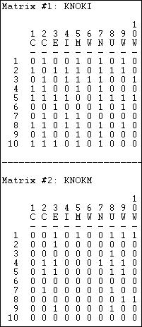
The most common structure for multi-plex data is a set of actor-by-actor matrices (or "slices"), one for each relation. Figure 16.1 shows the output of Data>Display for the Knoke social welfare organizations data set, which contains information on two (binary, directed) relations: information exchange (KNOKI), and money exchange (KNOKM).
Figure 16.1. Data>Display of Knoke multi-relational data structure
The two relations are stored as separate matrices, but within the same file. Many of the analysis tools in UCINET will process each matrix or "slice" of a multiple-matrix data file like the Knoke example. Data>Unpack can be used to remove individual matrices from a multiple matrix file; Data>Join can be used to create a multiple-matrix data set from separate single-matrix data files.
The multiple-matrix approach is most general, and allows us to record as many different relations as we wish by using separate matrices. Some matrices may be symmetric and others not; some may be binary, and others valued. A number of the tools that we will discuss shortly, however, will require that the data in the multiple matrices be of the same type (symmetric/asymmetric, binary/valued). So, often it will be necessary to do transformations on individual matrices before "reduction" and "combination" strategies can be applied.
A closely related multi-plex data structure is the "Cognitive social structure" or CSS. A CSS records the perceptions of a number of actors of the relations among a set of nodes. For example, we might ask each of Bob, Carol, Ted, and Alice to tell us who among them was friends with whom. The result would be four matrices of the same form (4 actors by 4 actors), reporting the same relation (who's friends with whom), but differing according to who is doing the reporting and perceiving.
CSS data have exactly the same form as standard actor-by-actor-by-slices. And some of the tools used for indexing CSS data are the same. Because of the unique nature of CSS data -- which focuses on complex perception of a single structure, instead of a single perception of a complex structure -- some additional tools may be applied (more, below).
A third, and rather different data structure is the multi-valued matrix. Suppose that the relations among actors were nominal (that is, qualitative, or "present-absent") but there were multiple kinds of relations each pair of actors might have - forming a nominal polyotomy. That is, each pair of actors had one (and only one) of several kinds of relations. For one example, relations among a set of actors might (in some populations) be coded as either "nuclear family co-member" or "co-workers" or "extended family member" or "co-religionist" or "none." For another example, we could combine multiple relations to create qualitative types: 1 = kin only, 2 = co-worker only, 3 = both kin and co-worker, and 4 = neither kin nor co-worker.
Nominal, but multi-valued, data combine information about multiplex relations into a single matrix. The values, however, don't represent strength, cost, or probability of a tie, but rather distinguish the qualitative type of tie that exists between each pair of actors. Recording data this way is efficient, and some algorithms in UCINET (e.g. Cateogrical REGE) can work directly with it. Often, though, data about multi-plex relations that has been stored in a single multi-valued matrix will need to be transformed before we can perform many network operations on it.
table of contentsFor relatively small networks, drawing graphs is the best way of "seeing" structure. The only new problem is how to represent multiple relations among actors. One approach is to use multiple lines (with different colors or styles) and over-lay one relation on another. Alternatively, one can "bundle" the relations into qualitative types and represent them with a single graph using line of different colors or styles (e.g. kin tie = red; work tie = blue; kin and work tie = green).
Netdraw has some useful tools for visualizing multiple relations among the same set of actors. If the data have been stored as multiple matrices within the same file, when that file is opened (Netdraw>File>Open>UCINET dataset>Network) a Ties dialog box will allow you to select which matrix to view (as well as to set cut-off values for visualizing valued data). This is useful for flipping back and forth between relations, with the nodes remaining in the same locations. Suppose, for example, we had stored ten matrices in a file, reflecting snapshots of relations in a network as it evolved over some period of time. Using the Ties dialog, we can "flip the pages" to see the network evolve.
An even more useful tool is found in Netdraw>Properties>Lines>Multi-relation selection. A drawing of the Knoke network with this dialog box visible is shown in figure 16.2.
Figure 16.2. NetDraw graph of Knoke information and money exchange networks
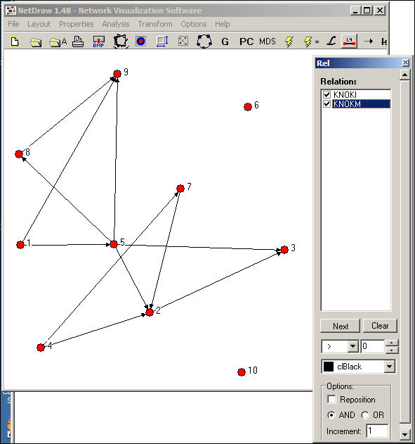
The Relations dialog box allows you to select which relations you would like to view, and whether to view the union ("or") or intersection ("and") of the ties. In our example, we've asked to see the pattern of ties among organizations that send both information and money to others.
table of contentsFor most analyses, the information about the multiple relations among actors will need to be combined into a single summary measure. One common approach is to combine the multiple relations into an index that reflects the quality (or type) of multi-plex relation.
Transform>Multiplex can be used to summarize multiple relations among actors into a qualitative multi-valued index. Suppose that we had measured two relations among Bob, Carol, Ted, and Alice. The first is a directed friendship nomination, and the second is a undirected spousal relation. These two four-by-four binary matrices have been packed into a single data file called BCTAjoin. The dialog for Transform>Multiplex is shown as figure 16.3.
Figure 16.3. Transform>multiplex dialog
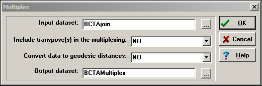
There are two choices here. Convert data to geodesic distances allows us to first convert each relation into a valued metric from the binary. We've chosen not to do this. Another choice is whether or not to Include transpose(s) in the multiplexing. For asymmetric data, selecting yes will cause the rows and the columns of the input matrix to be treated as separate relations in forming the qualitative combinations. Again, we've chosen not to do this (though it is a reasonable idea in many real cases).
Figure 16.4 shows the input file, which is composed of two "stacked" or "sliced" matrices representing friendship and spousal ties.
Figure 16.4. Transform>multiplex input
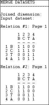
Figure 16.5 shows the resulting "typology" of kinds of relations among the actors, which has been generated as a multi-valued nominal index.
Figure 16.5. Transform>multiplex output
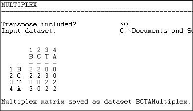
Where there is no tie in either matrix, the type "0" has been assigned. Where there is both a friendship and a spousal tie, the number "2" has been assigned; where there is a friendship tie, but no spousal tie, the number "3" has been assigned. There could have been an additional type (spousal tie, but no friendship) which would have been assigned a different number.
Combining multiple relations in this way yields a qualitative typology of the kinds of relations that exist among actors. An index of this type might be of considerable interest in describing the prevalence of the types in a population, and in selecting sub-graphs for closer analysis.
The operation Transform>Multigraph does the reverse of what Transform>Multiplex does. That is, if we begin with a multi-valued single matrix (as in figure 16.5), this operation will split the data and create a multiple matrix data file with one matrix for each "type" of relation. In the case of our example, Transform>Multigraph would generate two new matrices (one describing the "2" relation, and one describing the "3" relation).
In dealing with multiple relations among actors, we might also want to create a quantitative index that combines the relations. For example, we might suppose that if actors are tied by 4 different relations they share a "stronger" tie than if they share only 3 relations. But, there are many possible ways of creating indexes that capture different aspects or dimensions of the multiple relations among actors. Two tool-kits in UCINET support combining multiple matrices with a wide variety of built-in functions for capturing different aspects of the multi-relational data.
Transform>Matrix Operations>Matrix Operations>Between Datasets>Statistical Summaries provides some basic tools for creating a single valued matrix from multiple matrices. Figure 16.6 shows the dialog for this tool.
Figure 16.6. Dialog for between dataset matrix operations - statistical summaries
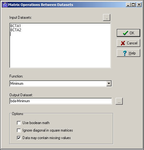
In the example, we've selected the two separate single-relation matrices for Bob, Carol, Ted, and Alice, and asked to create a new (single matrix) dataset called bda-Minimum. By selecting the Minimum function, we've chosen a rule that says: look at relations across the matrices, and summarize each pair-wise relation as the weakest one. For binary data, this is the same as the logical operation "and."
Also available in this dialog are Sum (which adds the values, element-wise, across matrices); Average (which computes the mean, element-wise, across matrices); Maximum (which selects the largest value, element-wise); and Element-wise Multiplication (which multiplies the elements across matrices). This is a pretty useful tool kit, and captures most of the ways in which quantitative indexes might be created (weakest tie, strongest tie, average tie, interaction of ties).
We might want to combine the information on multiple relations into a quantitative index by using logical operations instead of numeric. Figure 16.7 shows the dialog for Transform>Matrix Operations> Matrix Operations> Between Datasets>Boolean Combinations.
Figure 16.7. Dialog for between dataset matrix operations - Boolean combinations
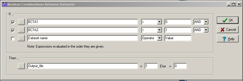
In this dialog, we've said: if there is a friendship tie and there is no spousal tie, then code the output relation as "1." Otherwise, code the output relation as "0." This is not a very sensible thing to do, but it illustrates the point that this tool can be used to perform basic logical operations to create valued (or binary) indexes that combine the information on multiple relations.
Suppose that I asked every member of the faculty of my department to fill out a questionnaire reporting on their perceptions of who likes whom among the faculty. We would be collecting "cognitive social structure" data; that is, reports from actors embedded in a network about the whole network. There is a very interesting research literature that explores the relationship between actor's positions in networks, and their perceptions of the network. For example, do actors have a bias toward perceiving their own positions as more "central" than other actors perception's of their centrality?
A cognitive social structure (CSS) dataset contains multiple actor-by-actor matrices. Each matrix reports on the full set of a single relation among all the actors, as perceived by a particular respondent. While we could use many of the tools discussed in the previous section to combine or reduce data like these into indexes, there are some special tools that apply to cognitive data. Figure 16.8 shows the dialog of Data>CSS, which provides access to some specialized tools for cognitive network research.
Figure 16.8. Dialog for Data>CSS
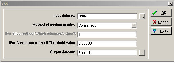
The key element here is the choice of Method for pooling graphs. In creating a single summary of the relations, we could select the perceptions of a single actor; or, we might want to focus on the perceptions of the pair of actors involved in each particular relationship; or we might want to combine the information of all of the actors in the network.
Slice selects the perception of one particular actor to represent the network (the dialog then asks, "which informant?"). If we had a particular expert informant we might choose his/her view of the network as a summary. Or, we could extract multiple different actors into different files. We might also extract actors based on some attribute (e.g. gender) and extract their graphs, then pool them by some other method.
Row LAS uses the data from each actor's row to be the row entry in the output matrix. That is, actor A's perceptions of his/her row values are used for row A in the output matrix; actor B's perceptions of his/her row values are used for row B in the output matrix. This uses each actor as the "informant" about their own out-ties.
Column LAS uses each actor's column to be the column entry in the output matrix. That is, each actor is being used as the "informant" regarding their own in-ties.
Intersection LAS constructs the output matrix by examining the entries of the particular pair of actors involved. For example, in the output matrix we would have an element that described the relation between Bob and Ted. We have data on how Bob, Ted, Carol, and Alice each perceive the relation of Bob and Ted. The LAS method focuses on only the two involved nodes (Bob and Ted) and ignores the others. The intersection method gives a "1" to the tie if both Bob and Ted say there is a tie, and a "0" otherwise.
Union LAS assigns a "1" to the pair-wise relation if either actor (i.e. either Bob or Ted) says there is a tie.
Median LAS selects the median of the two values for the B,T relation that are reported by B and by T. This is useful if the relation being examined is valued, rather than binary.
Consensus uses the perceptions of all actors to create the summary index. The perceptions of Bob, Carol, Ted, and Alice are summed, and if the sum is greater than a user specified cut-off value, "1" is assigned, else "0."
Average calculates the numerical average of all actor's perceptions of each pair-wise tie.
Sum calculates the sum of all actor's perceptions for each pair-wise tie.
The range of choices here suggests a fertile research area in how actors embedded in relations perceive those relations. The variety of indexing methods also suggests a number of interesting questions about, and methods for dealing with the reliability of network data when it is collected from embedded respondents.
table of contentsLet's suppose that we were looking at a single matrix on who was friends with whom. An obvious way of characterizing what we see is to classify the each pair as "friends" or "not friends." But now, let's extend our analysis one step further (or look at paths of length 2). Now each pair of actors could be characterized as friend, not friend, friend of friend, friend of not-friend, not-friend of friend, or not-friend of not friend. If we wanted to consider paths of length three...well, you get the idea.
The notion of a "role algebra" is to understand the relations between actors as realizations of the logically possible "compounds" of relations of selected path lengths. Most often in network analysis, we focus on path of length one (two actors are connected or not). But, sometimes it is useful to characterize a graph as containing more complex kinds of relations (friend of friend, not-friend of friend, etc.). Lists of these kinds of relations can be obtained by taking Boolean products of matrices (i.e. 0*0 = 0, 0*1 = 0, 1*0 = 0, and 1*1 = 1). When applied to single matrix, we raise a matrix to a power (multiply it by itself) and take the Boolean product; the result generates a matrix that tells us if there is a relation between each pair of nodes that is of a path length equal to the power. That is, to find whether each pair of actors is connected by the relation "friend of a friend" we take the Boolean product of the friendship matrix squared.
This (elegant, but rather mysterious) method of finding "compound relations" can be applied to multi-plex data as a way of identifying the kinds of relations that exist in a multi-plex graph. The Transform>Semigroup algorithm can be used to identify these more complex qualitative kinds of relations among nodes.
It is easier for most people to understand this with an example, than in the abstract. So let's do a somewhat extended examination of the Knoke data for both information and money ties.
If we consider just direct relations, there are two: organizations can be tied by information; organizations can be tied by money. What if consider relations at two steps (what are called "word lengths" in role algebra)? In addition to the original two relations, there are now four more:
These four new (two-step) relations among nodes are "words" of length two, or "compounds."
It is possible, of course, to continue to compound to still greater lengths. In most sociological analyses with only two types of ties, longer lengths are rarely substantively meaningful. With more kinds of ties, however, the number of types of compound relationships can become quite large quite quickly.
The tool Transform>Semigroup computes all of the logically possible compounded types of relations up to a word length (i.e. network distance) that the user specifies. It produces a log file that contains a "map" of the types of relations, as we see in Figure 16.9. It also produces, in a separate file, adjacency matrices for each of the types of relationships (Figures 16.10 and 16.11).
Figure 16.9. Semi-groups of word-length 2 for Knoke information and money networks
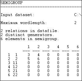
The output tells us that there were two relations (information and money). These were the "generators" that were used to create the types. Six possible compound relations were generated for the word-length 2 (identified down the left hand side). Relations 1 and 2 are information and money individually -- the original matrices. Relation 3 is a compound of information with itself; relation four is the compound of information with money, etc. The numbers (3, 4, 5, 6) are simply guides to which matrix in the output file refers to which relation.
From these new "types" of relations (which are compounds within and between the two types of ties) we can generate new adjacency matrices that show which pairs of actors are joined by each particular type of relation. These are presented as a series of adjacency matrices, as shown in figures 16.10 and continued in 16.11.
Figure 16.10. Relations tables for figure 16.9 (part 1)
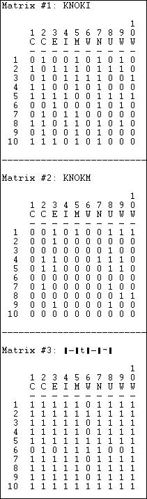
Matrix 1 is simply the original information matrix; matrix 2 is the original money matrix. Matrix 3 is the compound of information with information -- which actors are tied by a relationship "Ego sends information to someone who sends information to Alter?"
Figure 16.11. Relations tables for figure 16.9 (part 2)
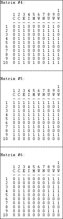
Matrix 4 is the compound of money with itself, or: "Ego sends money to someone who sends money to alter."
Matrices 5 and 6 are, in some ways, most interesting. While exchanging information for information and money for money are obvious ways in which a network can be integrated, its also possible that actors can be integrated by relations that involve both "apples" and "oranges." That is, I may send money, and receive information; I may send information, and receive money.
Role algebras have proven to be of particular value in the study of kinship relations, where across-generation (parent/child) ties are recorded in one matrix and within-generation relations are recorded in another. The various compounds (e.g. "child of child"; "child of brother") fairly easily capture the meaningful terms in kinship relations.
The actors in the kinds of networks that social scientists study are very frequently connected by more than one type of tie, simultaneously. That is, the relationship between any two actors may be multi-plex. In this chapter, we've introduced a few of the tools that are commonly used to help to make sense of the complex patterns of embedding that can emerge when there is more than one kind of tie operating simultaneously.
Multi-plex data are usually stored in a data structure of node-by-node matrices that are "stacked" as "slices" in a single file. Usually, these structures contain slices that measure different relations (e.g. money, information). However, the same data structure can be effectively used to store and work with multiple slices that show the state of the same network at multiple points in time, or the same network as perceived by different observers embedded in it (Cognitive social structures, or CSS). A compact way of storing information about multiple kinds of relations among actors in a single matrix, the multi-valued matrix, uses a number to reflect the qualitative type of relation that exists between two actors (e.g. none, money only, information only, information and money; or mutually exclusive "multiple choice" types like: kin, neighbor, co-worker).
With relatively small networks, and relatively small numbers of relations, graphs can be prepared that show the unions and intersections of multiple kinds of relations, or "animate" change over time in network structure.
Usually the information about multiple kinds of relations among actors is indexed by reducing the multiple ties into a single quantitative value that represents a summary across the separate relations (e.g. average tie strength, maximum, minimum). Alternatively, the information about different kinds of ties may be combined into more complex typologies using logical relations and "role algebra." A special set of tools for dealing with the unique features of CSS data was also discussed.
Many social network studies avoid the complexity of multi-plex data by focusing on a single relation, or by dealing with multiple relations separately. There is a good bit of virtue in this, for multi-plex analysis can be quite demanding (at least there are many plausible ways of approaching any multi-relational problem). Still, in some cases, engaging the full complexity of multi-plex data has paid huge returns. Our understanding of kinship structures, and our understanding of the positions of nation-states in the world system have been greatly enhanced by indexing actor's relational positions based on multiple and simultaneous ties.