13. Measures of similarity and structural equivalence
In this rather lengthy chapter we are going to do three things.
First, we will focus on how we can measure the similarity of actors in a network based on their relations to other actors. The whole idea of "equivalence" that we discussed in the last chapter is an effort to understand the pattern of relationships in a graph by creating classes, or groups of actors who are "equivalent" in one sense or another. All of the methods for identifying such groupings are based on first measuring the similarity or dissimilarity of actors, and then searching for patterns and simplifications. We will first review the most common approaches to indexing the similarities of actors based on their relations with other actors.
Second, we will very quickly look at two tools that are very commonly used for visualizing the patterns of similarity and dissimilarity/distance among actors. Multi-dimensional scaling and hierarchical cluster analysis are widely used tools for both network and non-network data. They are particularly helpful in visualizing the similarity or distance among cases, and for identifying classes of similar cases.
Third, we will examine the most commonly used approaches for finding structural equivalence classes. That is, methods for identifying groups of nodes that are similar in their patterns of ties to all other nodes. These methods (and those for other kinds of "equivalence" in the next two chapters) use the ideas of similarity/distance between actors as their starting point; and, these methods most often use clustering and scaling as a way of visualizing results. In addition, the "block model" is also commonly used to describe structural similarity classes.
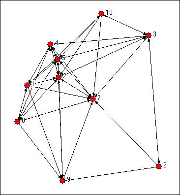
We might try to assess which nodes are most similar to which other nodes intuitively by looking at a graph. We would notice some important things. It would seem that actors 2,5, and 7 might be structurally similar in that they seem to have reciprocal ties with each other and almost everyone else. Actors 6, 8, and 10 are "regularly" similar in that they are rather isolated; but they are not structurally similar because they are connected to quite different sets of actors. But, beyond this, it is really rather difficult to assess equivalence rigorously by just looking at a diagram.
Figure 13.1. Knoke directed information network
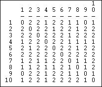
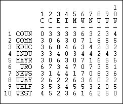
We can be a lot more precise in assessing similarity if we use the matrix representation of the network instead of the diagram. This also lets us use the computer to do some of the quite tedious jobs involved in calculating index numbers to assess similarity. The original data matrix has been reproduced below as figure 13.2. Many of the features that were apparent in the diagram are also easy to grasp in the matrix. If we look across the rows and count out-degrees, and if we look down the columns (to count in-degree) we can see who the central actors are and who are the isolates. But, even more generally, we can see that two actors are structurally equivalent to extent that the profile of scores in their rows and columns are similar. Finding automorphic equivalence and regular equivalence is not so simple. But, since these other forms are less restrictive (and hence simplifications of the structural classes), we begin by measuring how similar each actor's ties are to all other actors.
Figure 13.2. Adjacency matrix for Knoke information network
| 1 Coun | 2 Comm | 3 Educ | 4 Indu | 5 Mayr | 6 WRO | 7 News | 8 UWay | 9 Welf | 10 West | |
| 1 Coun |
--- |
1 |
0 |
0 |
1 |
0 |
1 |
0 |
1 |
0 |
| 2 Comm |
1 |
--- |
1 |
1 |
1 |
0 |
1 |
1 |
1 |
0 |
| 3 Educ |
0 |
1 |
--- |
1 |
1 |
1 |
1 |
0 |
0 |
1 |
| 4 Indu |
1 |
1 |
0 |
--- |
1 |
0 |
1 |
0 |
0 |
0 |
| 5 Mayr |
1 |
1 |
1 |
1 |
--- |
0 |
1 |
1 |
1 |
1 |
| 6 WRO |
0 |
0 |
1 |
0 |
0 |
--- |
1 |
0 |
1 |
0 |
| 7 News |
0 |
1 |
0 |
1 |
1 |
0 |
--- |
0 |
0 |
0 |
| 8 UWay |
1 |
1 |
0 |
1 |
1 |
0 |
1 |
--- |
1 |
0 |
| 9 Welf |
0 |
1 |
0 |
0 |
1 |
0 |
1 |
0 |
--- |
0 |
| 10 West |
1 |
1 |
1 |
0 |
1 |
0 |
1 |
0 |
0 |
--- |
Two actors may be said to be structurally equivalent to if they have the same patterns of ties with other actors. This means that the entries in the rows and columns for one actor are identical to those of another. If the matrix were symmetric, we would need only to scan pairs of rows (or columns). But, since these data are on directed ties, we should examine the similarity of sending and receiving of ties (of course, we might be interested in structural equivalence with regard to only sending, or only receiving ties). We can see the similarity of the actors if we expand the matrix in figure 13.2 by listing the row vectors followed by the column vectors for each actor as a single column, as we have in figure 13.3.
Figure 13.3. Concatenated row and column adjacencies for Knoke
information network
| 1 Coun | 2 Comm | 3 Educ | 4 Indu | 5 Mayr | 6 WRO | 7 News | 8 UWay | 9 Welf | 10 West |
|
--- |
1 |
0 |
1 |
1 |
0 |
0 |
1 |
0 |
1 |
|
1 |
--- |
1 |
1 |
1 |
0 |
1 |
1 |
1 |
1 |
|
0 |
1 |
--- |
0 |
1 |
1 |
0 |
0 |
0 |
1 |
|
0 |
1 |
1 |
--- |
1 |
0 |
1 |
1 |
0 |
0 |
|
1 |
1 |
1 |
1 |
--- |
0 |
1 |
1 |
1 |
1 |
|
0 |
0 |
1 |
0 |
0 |
--- |
0 |
0 |
0 |
0 |
|
1 |
1 |
1 |
1 |
1 |
1 |
--- |
1 |
1 |
1 |
|
0 |
1 |
0 |
0 |
1 |
0 |
0 |
--- |
0 |
0 |
|
1 |
1 |
0 |
0 |
1 |
1 |
0 |
1 |
--- |
0 |
|
0 |
0 |
1 |
0 |
1 |
0 |
0 |
0 |
0 |
--- |
|
--- |
1 |
0 |
0 |
1 |
0 |
1 |
0 |
1 |
0 |
|
1 |
--- |
1 |
1 |
1 |
0 |
1 |
1 |
1 |
0 |
|
0 |
1 |
--- |
1 |
1 |
1 |
1 |
0 |
0 |
1 |
|
1 |
1 |
0 |
--- |
1 |
0 |
1 |
0 |
0 |
0 |
|
1 |
1 |
1 |
1 |
--- |
0 |
1 |
1 |
1 |
1 |
|
0 |
0 |
1 |
0 |
0 |
--- |
1 |
0 |
1 |
0 |
|
0 |
1 |
0 |
1 |
1 |
0 |
--- |
0 |
0 |
0 |
|
1 |
1 |
0 |
1 |
1 |
0 |
1 |
--- |
1 |
0 |
|
0 |
1 |
0 |
0 |
1 |
0 |
1 |
0 |
--- |
0 |
|
1 |
1 |
1 |
0 |
1 |
0 |
1 |
0 |
0 |
--- |
The ties of each actor (both out and in) are now represented as a column of data. We can now measure the similarity of each pair of columns to index the similarity of the two actors; forming a pair-wise matrix of similarities. We could also get at the same idea in reverse, by indexing the dissimilarity or "distance" between the scores in any two columns.
There are any number of ways to index similarity and distance. In the next two sections we'll briefly review the most commonly used approaches when the ties are measured as values (i.e. strength or cost or probability) and as binary.
The goal here is to create an actor-by-actor matrix of the similarity (or distance) measures. Once we have done this, we can apply other techniques for visualizing the similarities in the actor's patterns of relations with other actors.
A common approach for indexing the similarity of two valued variables is the degree of linear association between the two. Exactly the same approach can be applied to the vectors that describe the relationship strengths of two actors to all other actors. As with any measures of linear association, linearity is a key assumption. It is often wise, even when data are at the interval level (e.g. volume of trade from one nation to all others) to consider measures with weaker assumptions (like measures of association designed for ordinal variables).
The correlation measure of similarity is particularly useful when the data on ties are "valued," that is, tell us about the strength and direction of association, rather than simple presence or absence. Pearson correlations range from -1.00 (meaning that the two actors have exactly the opposite ties to each other actor), through zero (meaning that knowing one actor's tie to a third party doesn't help us at all in guessing what the other actor's tie to the third party might be), to +1.00 (meaning that the two actors always have exactly the same tie to other actors - perfect structural equivalence). Pearson correlations are often used to summarize pair-wise structural equivalence because the statistic (called "little r") is widely used in social statistics. If the data on ties are truly nominal, or if density is very high or very low, correlations can sometimes be a little troublesome, and matches (see below) should also be examined. Different statistics, however, usually give very much the same answers. Figure 13.4 shows the correlations of the ten Knoke organization's profiles of in and out information ties. We are applying correlation, even though the Knoke data are binary. The UCINET algorithm Tools>Similarities will calculate correlations for rows or columns.
Figure 13.4. Pearson correlations of rows (sending) for Knoke information network
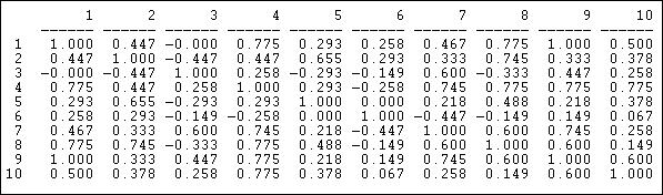
We can see, for example, that node 1 and node 9 have identical patterns of ties; there is a moderately strong tendency for actor 6 to have ties to actors that actor 7 does not, and vice versa.
The Pearson correlation measure does not pay attention to the overall prevalence of ties (the mean of the row or column), and it does not pay attention to differences between actors in the variances of their ties. Often this is desirable - to focus only on the pattern, rather than the mean and variance as aspects of similarity between actors.
Often though, we might want our measure of similarity to reflect not only the
pattern of ties, but also differences among actors in their overall tie
density. Tools>Similarities will
also calculate the covariance matrix. If we want to include
differences in variances across actors as aspects of (dis)similarity, as well as
means, the cross-product ratio calculated in Tools>Similarities
might be used.
table of contents
An alternative approach to linear correlation (and its relatives) is to measure the "distance" or "dissimilarity" between the tie profiles of each pair of actors. Several "distance" measures are fairly commonly used in network analysis, particularly the Euclidean distance or squared Euclidean distance. These measures are not sensitive to the linearity of association and can be used with either valued or binary data.
Figure 13.5 shows the Euclidean distances among the Knoke organizations calculated using Tools>Dissimilarities and Distances>Std Vector dissimilarities/distances.
Figure 13.5. Euclidian distances in sending for Knoke information network
The Euclidean distance between two vectors is equal to the square root of the sum of the squared differences between them. That is, the strength of actor A's tie to C is subtracted from the strength of actor B's tie to C, and the difference is squared. This is then repeated across all the other actors (D, E, F, etc.), and summed. The square root of the sum is then taken.
A closely related measure is the "Manhattan" or block distance between the two vectors. This distance is simply the sum of the absolute difference between the actor's ties to each alter, summed across the alters.
table of contentsIf the information that we have about the ties among our actors is binary, correlation and distance measures can be used, but may not be optimal. For data that are binary, it is more common to look at the vectors of two actor's ties, and see how closely the entries in one "match" the entries in the other.
There are a several useful measures of tie profile similarity based on the matching idea that are calculated by Tools>Similarities
A very simple and often effective approach to measuring the similarity of two tie profiles is to count the number of times that actor A's tie to alter is the same as actor B's tie to alter, and express this as a percentage of the possible total.
Figure 13.6 shows the result for the columns (information receiving) relation of the Knoke bureaucracies.
Figure 13.6 Proportion of matches for Knoke information receiving
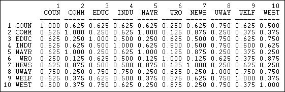
These results show similarity in a way that is quite easy to interpret. The number .625 in the cell 2,1 means that, in comparing actor #1 and #2, they have the same tie (present or absent) to other actors 62.5% of the time. The measure is particularly useful with multi-category nominal measures of ties; it also provides a nice scaling for binary data.
In some networks connections are very sparse. Indeed, if one were looking at ties of personal acquaintance in very large organizations, the data might have very low density. Where density is very low, the "matches" "correlation" and "distance" measures can all show relatively little variation among the actors, and may cause difficulty in discerning structural equivalence sets (of course, in very large, low density networks, there may really be very low levels of structural equivalence).
One approach to solving this problem is to calculate the number of times that both actors report a tie (or the same type of tie) to the same third actors as a percentage of the total number of ties reported. That is, we ignore cases where neither X or Y are tied to Z, and ask, of the total ties that are present, what percentage are in common. Figure 13.7 shows the Jaccard coefficients for information receiving in the Knoke network, calculated using Tools>Similarities, and selecting "Jaccard."
Figure 13.7 Jaccard coefficients for information receiving profiles in Knoke network
Percent of Positive Matches (Jaccard coefficients)

         1     2     3     4     5     6     7     8     9    10
       COUN  COMM  EDUC  INDU  MAYR   WRO  NEWS  UWAY  WELF  WEST
       ----- ----- ----- ----- ----- ----- ----- ----- ----- -----
  1    1.00
  2    0.54  1.00
  3    0.46  0.31  1.00
  4    0.60  0.54  0.42  1.00
  5    0.50  0.93  0.38  0.50  1.00
  6    0.18  0.27  0.11  0.18  0.25  1.00
  7    0.58  0.64  0.54  0.55  0.60  0.08  1.00
  8    0.67  0.46  0.50  0.67  0.43  0.20  0.38  1.00
  9    0.67  0.36  0.50  0.55  0.33  0.11  0.64  0.56  1.00
 10    0.40  0.43  0.44  0.60  0.36  0.38  0.31  0.50  0.36  1.00
Again the same basic picture emerges. The uniqueness of actor #6, though is emphasized. Actor six is more unique by this measure because of the relatively small number of total ties that it has -- this results in a lower level of similarity when "joint absence" of ties are ignored. Where data are sparse, and where there are very substantial differences in the degrees of points, the positive match coefficient is a good choice for binary or nominal data.
Another interesting "matching" measure is the Hamming distance, shown in figure 13.8.
Figure 13.8. Hamming distances of information receiving in Knoke network
The Hamming distance is the number of entries in the vector for one actor that would need to be changed in order to make it identical to the vector of the other actor. These differences could be either adding or dropping a tie, so the Hamming distance treats joint absence as similarity.
With some inventiveness, you can probably think of some other reasonable ways of indexing the degree of structural similarity between actors. You might look at the program "Proximities" by SPSSx, which offers a large collection of measures of similarity. The choice of a measure should be driven by a conceptual notion of "what about" the similarity of two tie profiles is most important for the purposes of a particular analysis. Often, frankly, it makes little difference, but that is hardly sufficient grounds to ignore the question.
In the section above, we've seen how the degree of similarity or distance between two actors patterns of ties with other actors can be measured and indexed. Once this is done, then what?
It is often useful to examine the similarities or distances to try to locate groupings of actors (that is, larger than a pair) who are similar. By studying the bigger patterns of which groups of actors are similar to which others, we may also gain some insight into "what about" the actor's positions is most critical in making them more similar or more distant.
Two tools that are commonly used for visualizing patterns of relationships among variables are also very helpful in exploring social network data. When we have created a similarity or distance matrix describing all the pairs of actors, we can study the similarity of differences among "cases" relations in the same way that we would study similarities among attributes.
In the next two sections we will show very brief examples of how multi-dimensional scaling and hierarchical cluster analysis can be used to identify patterns in actor-by-actor similarity/distance matrices. Both of these tools are widely used in non-network analysis; there are large and excellent literatures on the many important complexities of using these methods. Our goal here is just to provide just a very basic introduction.
Agglomerative hierarchical clustering of nodes on the basis of the similarity of their profiles of ties to other cases provides a "joining tree" or "dendogram" that visualizes the degree of similarity among cases - and can be used to find approximate equivalence classes.
Tools>Cluster>Hierarchical proceeds by initially placing each case in its own cluster. The two most similar cases (those with the highest measured similarity index) are then combined into a class. The similarity of this new class to all others is then computed on the basis of one of three methods. On the basis of the newly computed similarity matrix, the joining/recalculation process is repeated until all cases are "agglomerated" into a single cluster. The "hierarchical" part of the method's name refers to the fact that once a case has been joined into a cluster, it is never re-classified. This results in clusters of increasing size that always enclose smaller clusters.
The "Average" method computes the similarity of the average scores in the newly formed cluster to all other clusters; the "Single-Link" method (a.k.a. "nearest neighbor") computes the similarities on the basis of the similarity of the member of the new cluster that is most similar to each other case not in the cluster. The "Complete-Link" method (a.k.a. "farthest neighbor") computes similarities between the member of the new cluster that is least similar to each other case not in the cluster. The default method is to use the cluster average; single-link methods will tend to give long-stringy joining diagrams; complete-link methods will tend to give highly separated joining diagrams.
The Hamming distance in information sending in the Knoke network was computed as shown in the section above, and the results were stored as a file. This file was then input to Tools>Cluster>Hierarchical. We specified that the "average" method was to be used, and that the data were "dissimilarities." The results are shown as figure 13.9.
Figure 13.9. Clustering of Hamming distances of information sending in the Knoke network
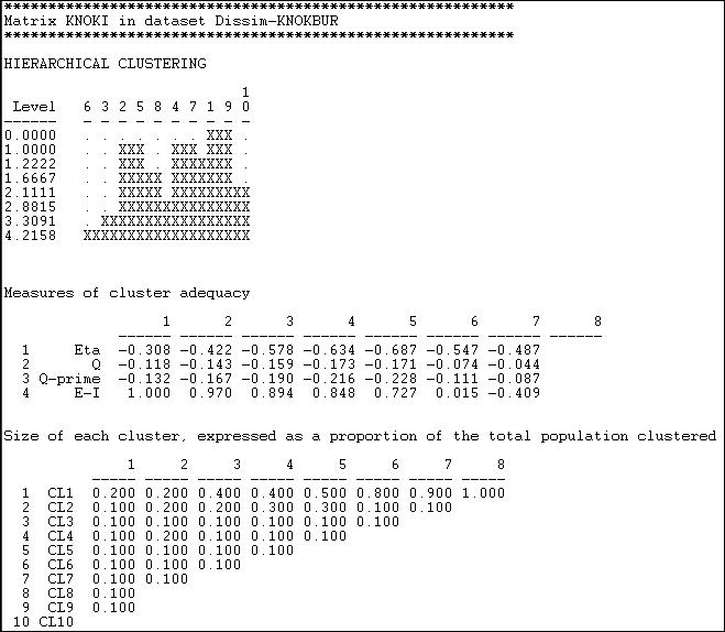
The first graphic shows that nodes 1 and 9 were the most similar, and joined first. The graphic, by the way, can be rendered as a more polished dendogram using Tools>Dendogram>Draw on data saved from the cluster tool. At the next step, there are three clusters (cases 2 and 5, 4 and 7, and 1 and 9). The joining continues until (at the 8th step) all cases are agglomerated into a single cluster. This gives a clear picture of the similarity of cases, and the groupings or classes of cases. But there are really eight pictures here (one for each step of the joining). Which is the "right" solution?
Again, there is no single answer. Theory and a substantive knowledge of the processes giving rise to the data are the best guide. The second panel "Measures of cluster adequacy" can be of some assistance. There are a number of indexes here, and most will (usually) give the similar answers. As we move from the right (higher steps or amounts of agglomeration) to the left (more clusters, less agglomeration) fit improves. The E-I index is often most helpful, as it measures the ratio of the numbers of ties within the clusters to ties between clusters. Generally, the goal is to achieve classes that are highly similar within, and quite distinct without. Here, one might be most tempted by the solution of the 5th step of the process (clusters of 2+5, 4+7+1+9, and the others being single-item clusters).
To be meaningful, clusters should also contain a reasonable percentage of the cases. The last panel shows information on the relative sizes of the clusters at each stage. With only 10 cases to be clustered in our example, this is not terribly enlightening here.
UCINET provides two additional cluster analysis tools that we won't discuss at any length here -- but which you may wish to explore. Tools>Cluster>Optimization allows the user to select, a priori, a number of classes, and then uses the chosen cluster analysis method to optimally fit cases to classes. This is very similar to the structural optimization technique we will discuss below. Tools>Cluster>Cluster Adequacy takes a user-supplied classification (a partition, or attribute file), fits the data to it, and reports on the goodness of fit.
Usually our goal in equivalence analysis is to identify and visualize "classes" or clusters of cases. In using cluster analysis, we are implicitly assuming that the similarity or distance among cases reflects as single underlying dimension. It is possible, however, that there are multiple "aspects" or "dimensions" underlying the observed similarities of cases. Factor or components analysis could be applied to correlations or covariances among cases. Alternatively, multi-dimensional scaling could be used (non-metric for data that are inherently nominal or ordinal; metric for valued).
MDS represents the patterns of similarity or dissimilarity in the tie profiles among the actors (when applied to adjacency or distances) as a "map" in multi-dimensional space. This map lets us see how "close" actors are, whether they "cluster" in multi-dimensional space, and how much variation there is along each dimension.
Figures 13.10 and 13.11 show the results of applying Tools>MDS>Non-Metric MDS to the raw adjacency matrix of the Knoke information network, and selecting a two-dimensional solution.
Figure 13.10. Non-metric MDS two-dimensional coordinates of Knoke information adjacency
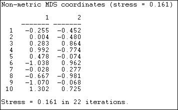
"Stress" is a measure of badness of fit. In using MDS, it is a good idea to look at a range of solutions with more dimensions, so you can assess the extent to which the distances are uni-dimensional. The coordinates show the location of each case (1 through 10) on each of the dimensions. Case one, for example, is in the lower left quadrant, having negative scores on both dimension 1 and dimension 2.
The "meaning" of the dimensions can sometimes be assessed by comparing cases that are at the extreme poles of each dimension. Are the organizations at one pole "public" and those at the other "private?" In analyzing social network data, it is not unusual for the first dimension to be simply the amount of connection or the degree of the nodes.
Figure 13.11. Two-dimensional map of non-metric MDS of Knoke information adjacency
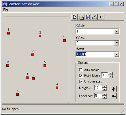
Figure 13.11 graphs the nodes according to their coordinates. In this map, we are looking for meaningful tight clusters of points to identify cases that are highly similar on both dimensions. In our example, there is very little such similarity (save, perhaps, nodes 1 and 2).
Clustering and scaling tools can be useful in many kinds of network analysis. Any measure of the relations among nodes can be visualized using these methods -- adjacency, strength, correlation and distance are most commonly examined.
These tools are also quite useful for examining equivalence. Most methods for assessing equivalence generate actor-by-actor measures of closeness or similarity in the tie profiles (using different rules, depending on what type of equivalence we are trying to measure). Cluster and MDS are often quite helpful in making sense of the results.
table of contentsTwo actors that are structurally equivalent have the same ties to all other actors -- they are perfectly substitutable or exchangeable. In "real" data, exact equivalence may be quite rare, and it may be meaningful to measure approximate equivalence. There are a several approaches for examining the pattern of similarities in the tie-profiles of actors, and for forming structural equivalence classes.
One very useful approach is to apply cluster analysis to attempt to discern how many structural equivalence sets there are, and which actors fall within each set. We will examine two more common approaches -- CONCOR, and numerical optimization by tabu search.
What the similarity matrix and cluster analysis do not tell us is what similarities make the actors in each set "the same" and which differences make the actors in one set "different" from the actors in another. A very useful approach to understanding the bases of similarity and difference among sets of structurally equivalent actors is the block model, and a summary based on it called the image matrix. Both of these ideas have been explained elsewhere. We will take a look at how they can help us to understand the results of CONCOR and tabu search.
Cluster analysis is a natural method for exploring structural equivalence. Two actors who have the similar patterns of ties to other actors will be joined into a cluster, and hierarchical methods will show a "tree" of successive joining.
Network>Roles & Positions>Structural>Profile can perform a variety of kinds of cluster analysis for assessing structural equivalence. Figure 13.12 shows a typical dialog for this algorithm.
Figure 13.12. Dialog of Network>Roles & Positions>Structural>Profile
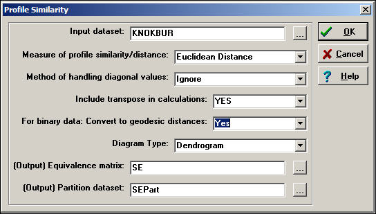
Depending on how the relations between actors have been measured, several common ways of constructing the actor-by-actor similarity or distance matrix are provided (correlations, Euclidean distances, total matches, or Jaccard coefficients). Should you desire a different measure of similarity, you can construct it elsewhere (e.g. Tools>Similarities), save the result, and apply cluster analysis directly (i.e. Tools>Cluster).
There are some other important choices. One is, what to do with the items in the similarity matrix that index the similarity of an actor to themselves (i.e. the diagonal values)? One choice ("Retain") includes the similarity of a node with itself; another choice ("Ignore") excludes diagonal elements from the calculation of similarity or difference. The default method ("Reciprocal") replaces the diagonal element for both cases with the tie that exists between the cases.
One may "Include transpose" or not. If the data being examined are symmetric (i.e. a simple graph, not a directed one), then the transpose is identical to the matrix, and shouldn't be included. For directed data, the algorithm will, by default, calculate similarities on the rows (out-ties) but not in-ties. If you want to include the full profile of both in and out ties for directed data, you need to include the transpose.
If you are working with a raw adjacency matrix, similarity can be computed on the tie profile (probably using a match or Jaccard approach). Alternatively, the adjacencies can be turned into a valued measure of dissimilarity by calculating geodesic distances (in which case correlations or Euclidean distances might be chosen as a measure of similarity).
Figure 13.13 shows the results of the analysis described in the dialog.
Figure 13.13. Profile similarity of geodesic distances of rows and columns of Knoke information network
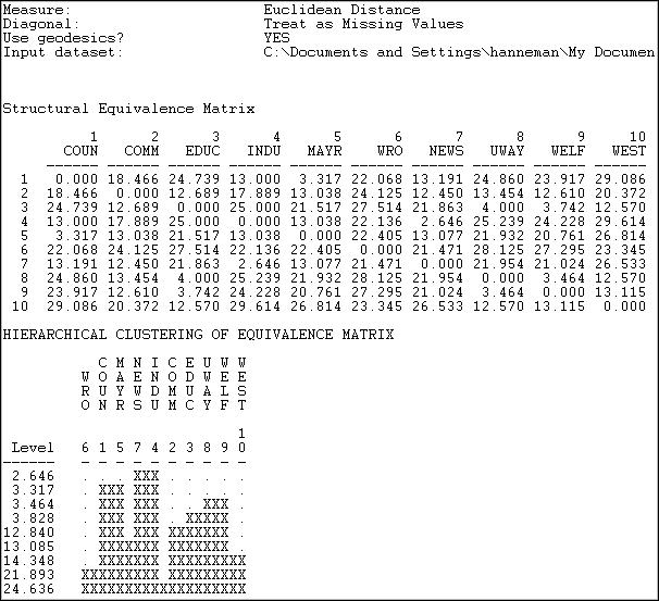
The first panel shows the structural equivalence matrix - or the degree of similarity among pairs of actors (in this case, dis-similarity, since we chose to analyze Euclidean distances).
The second panel shows a rough character-mapped graphic of the clustering. Here we see that actors 7 and 4 are most similar; a second cluster is formed by actors 1 and 5; a third by actors 8 and 9). This algorithm also provides a more polished presentation of the result as a dendogram in a separate window, as shown in Figure 13.14.
Figure 13.14. Dendogram of structural equivalence data (see figure 13.13)
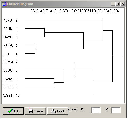
There are no exact structural equivalences in the example data. That is, there are no two cases that have identical ties to all other cases. The dendogram can be particularly helpful in locating groupings of cases that are sufficiently equivalent to be treated as classes. The measures of clustering adequacy in Tools>Cluster can provide additional guidance.
Two other approaches, CONCOR and optimization, follow a somewhat different logic than clustering. In both of these methods, partitions or approximate equivalence classes are set up first (the user selects how many), and the cases are allocated to these classes by numerical techniques designed to maximize similarity within classes.
CONCOR is an approach that has been used for quite some time. Although the algorithm of concor is now regarded as a bit peculiar, the technique usually produces meaningful results.
CONCOR begins by correlating each pair of actors (as we did above). Each row of this actor-by-actor correlation matrix is then extracted, and correlated with each other row. In a sense, the approach is asking "how similar is the vector of similarities of actor X to the vector of similarities of actor Y?" This process is repeated over and over. Eventually the elements in this "iterated correlation matrix" converge on a value of either +1 or -1 (if you want to convince yourself, give it a try!).
CONCOR then divides the data into two sets on the basis of these correlations. Then, within each set (if it has more than two actors) the process is repeated. The process continues until all actors are separated (or until we lose interest). The result is a binary branching tree that gives rise to a final partition.
For illustration, we have asked CONCOR to show us the groups that best satisfy this property when we believe that there are four groups in the Knoke information data. We used Network>Roles & Positions>Structural>CONCOR, and set the depth of splits = 2 (that is, divide the data twice). All blocking algorithms require that we have a prior idea about how many groups there are. The results are shown in figure 13.15.
Figure 13.15. CONCOR on Knoke information matrix with two splits
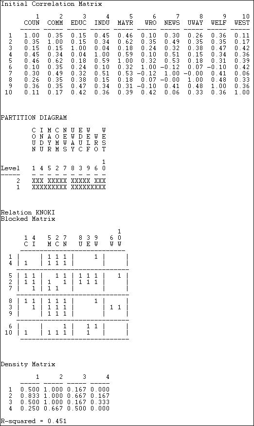
The first panel shows the correlations of the cases. We included the transpose, so these correlations are based on both sending and receiving of ties. Our data, however, are binary, so the use of the correlation coefficient (and CONCOR) should be treated with caution.
The second panel shows the two splits. In the first division, the two groups {1, 4, 5, 2, 7} and {8, 3, 9, 6, 10} were formed. On the second split these were sub-divided into {1, 4}, {5, 2,7}, {8, 3, 9}, and {6, 10}.
The third panel (the "Blocked Matrix") shows the permuted original data. The result here could be simplified further by creating a "block image" matrix of the four classes by the four classes, with "1" in high density blocks and "0" in low density blocks - as in figure 13.15.
Figure 13.15. Block image of CONCOR results
| [1] | [2] | [3] | [4] | |
| [1] |
0 |
1 |
0 |
0 |
| [2] |
1 |
1 |
1 |
0 |
| [3] |
1 |
1 |
0 |
0 |
| [4] |
0 |
1 |
1 |
0 |
The goodness of fit of a block model can be assessed by correlating the permuted matrix (the block model) against a "perfect" model with the same blocks (i.e. one in which all elements of one blocks are ones, and all elements of zero blocks are zeros). For the CONCOR two-split (four group) model, this r-squared is .451. That is, about 1/2 of the variance in the ties in the CONCOR model can be accounted for by a "perfect" structural block model. This might be regarded as OK, but is hardly a wonderful fit (there is no real criterion for what is a good fit).
The block model and its image also provide a description of what it means when we say "the actors in block one are approximately structurally equivalent." Actors in equivalence class one are likely to send ties to all actors in block two, but no other block. Actors in equivalence class one are likely to receive ties from all actors in blocks 2 and 3. So, we have not only identified the classes, we've also described the form of the relations that makes the cases equivalent.
This method of blocking has been developed more recently, and relies on extensive use of the computer. Tabu search uses a more modern (and computer intensive) algorithm than CONCOR, but is trying to implement the same idea of grouping together actors who are most similar into a block. Tabu search does this by searching for sets of actors who, if placed into a blocks, produce the smallest sum of within-block variances in the tie profiles. That is, if actors in a block have similar ties, their variance around the block mean profile will be small. So, the partitioning that minimizes the sum of within block variances is minimizing the overall variance in tie profiles. In principle, this method ought to produce results similar (but not necessarily identical) to CONCOR. In practice, this is not always so. Here (figure 13.16) are the results of Network>Roles & Positions>Structural>Optimization>Binary applied to the Knoke information network, and requesting four classes. A variation of the technique for valued data is available as Network>Roles & Positions>Structural>Optimization>Valued.
Figure 13.16 Optimized four-block solution for structural equivalence of Knoke information network.
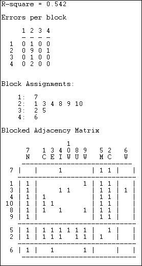
The overall correlation between the actual scores in the blocked matrix, and a "perfect" matrix composed of only ones and zeros is reasonably good (.544).
The suggested partition into structural equivalence classes is {7}, {1, 3, 4, 10, 8, 9}, {5, 2}, and {6}.
We can now also describe the positions of each of the classes. The first class (actor 7) has dense sending ties to the third (actors 5 and 2); and receives information from all three other classes. The second, and largest, class sends information to the first and the third class, and receives information from the third class. The third class (5 and 2) send information to the first and second class, as well as among themselves; they receive information from the second class. The last class (actor 6), sends to the first class, but receives from none.
This last analysis illustrates most fully the primary goals of an analysis of structural equivalence:
1) how many equivalence classes, or approximate equivalence classes are there?
2) how good is the fit of this simplification into equivalence classes in summarizing the information about all the nodes?
3) what is the position of each class, as defined by its relations to the other classes?
In this section we have discussed the idea of "structural equivalence" of actors, and seen some of the methodologies that are most commonly used to measure structural equivalence, find patterns in empirical data, and describe the sets of "substitutable" actors.
Structural equivalence of two actors is the degree to which the two actors have the same profile of relations across alters (all other actors in the network). Exact structural equivalence is rare in most social structures (one interpretation of exact structural equivalence is that it represents systematic redundancy of actors; which may be functional in some way to the network).
While it is sometimes possible to see patterns of structural equivalence "by eye" from an adjacency matrix or diagram, we almost always use numerical methods. Numerical methods allow us to deal with multiplex data, large numbers of actors, and valued data (as well as the binary type that we have examined here).
The first step in examining structural equivalence is to produce a "similarity" or a "distance" matrix for all pairs of actors. This matrix summarizes the overall similarity (or dissimilarity) of each pair of actors in terms of their ties to alters. While there are many ways of calculating such index numbers, the most common are the Pearson Correlation, the Euclidean Distance, the proportion of matches (for binary data), and the proportion of positive matches (Jaccard coefficient, also for binary data).
A number of methods may be used to identify patterns in the similarity or distance matrix, and to describe those patterns. Cluster analysis groups together the two most similar actors, recalculates similarities, and iterates until all actors are combined. What is produced is a "joining sequence" or map of which actors fall into a hierarchy of increasingly inclusive (and hence less exactly equivalent) groups. Multi-dimensional scaling and factor analysis can be used to to identify what aspects of the tie profiles are most critical to making actors similar or different, and can also be used to identify groups. Groupings of structurally equivalent actors can also be identified by the divisive method of iterating the correlation matrix of actors (CONCOR), and by the direct method of permutation and search for perfect zero and one blocks in the adjacency matrix (Optimization by Tabu search).
Once the number of groupings that are useful has been determined, the data can be permuted and blocked , and images calculated. These techniques enable us to get a rather clear picture of how the actors in one set are "approximately equivalent" and why different sets of actors are different. That is, they enable us to describe the meaning of the groups, and the place of group members in the overall network in a general way.
Structural equivalence analysis often produces interesting and revealing findings about the patterns of ties and connections among the individual actors in a network. The structural equivalence concept aims to operationalize the notion that actors may have identical or nearly identical positions in a network -- and hence be directly "substitutable" for one another. An alternative interpretation is that actors who are structurally equivalent face nearly the same matrix of constraints and opportunities in their social relationships.
Sociological analysis is not really about individual people. And, structural analysis, is primarily concerned with the more general and abstract idea of the roles or positions that define the structure of the group -- rather than the locations of specific actors with regard to specific others. For such analysis, we turn to a related set of tools for studying replicate sub structures ("automorphic equivalence") and social roles ("regular equivalence").