Spatial Dynamics of Human Populations: Some Basic Models
Robert A. Hanneman
(robert.hanneman@ucr.edu)
Department of Sociology
University of California, Riverside
Jason Martinez
California State University, San Bernardino
2005
Schelling's model of residential segregation
In most human populations that are composed of "sub-populations" there are variable tendencies toward spatial segregation. The distribution of persons by "race" in the United States, for example, displays very high levels of segregation. Physical separation of groups that are recognized as "different" from one another tends to re-enforce perceptions of difference, and may contribute to the formation of negative or antagonistic beliefs about "them." Attitudes that express a preference for interaction with members of one's own group (and, consequently, a preference to avoid interaction with the other group) are called "homophily."
The positive feedback cycle of segregation - prejudice - in-group preference can be found in most human populations, with greatly variation in what are regarded as meaningful differences -- gender, age, "race," ethnicity, language, sexual preference, religion, etc.
Once a cycle of separation-prejudice-discrimination-separation has begun, it has a self-sustaining momentum. But how do such dynamics emerge? There are, in fact, quite a number of social processes that can generate (or retard, and sometimes reverse) these dynamics. In this page, we will explore one very interesting model advanced by Thomas Schelling (Schelling, Thomas C. 1971. "Dynamic Models of Segregation." Journal of Mathematical Sociology. 1:143-186). This model is of particular interest in the current context, because the dynamic process involved is explicitly spatial.
Let's examine a very simple case in which members of two social groups ("reds" and "greens") occupy random spaces in a rectangular grid. There are also a number of unoccupied locations. Let's further suppose that the two sub-populations are equal in numbers (this isn't an essential assumption).
Assume that all "reds" are quite "tolerant" of greens. They are willing to live in "mixed neighborhoods" in which both groups are proportionally represented. Assume that "greens" feel the same way. However, let's also assume that, while members of each group are tolerant of the other, that no one wants to be a "minority" in their neighborhood. That is, greens are happy to live in a neighborhood with up to 50% reds -- but not more than that; reds feel the same way about the presence of greens.
If any member of the population finds them self in a neighborhood where they are not a minority, they are happy. But, if they find them self in a neighborhood where they are a minority, they move to a randomly chosen "open" square.
What will happen when we set this process in motion?
You may be thinking: reds and greens are randomly distributed, and all are tolerant of living in neighborhoods that are (on the average) representative of the population as a whole. So, won't everyone be happy? And, if they are, then the "dynamic" should be that no one moves.
This is not what happens. See if you can reason why this might be. And then, read on.
Table of contentsWe present three different versions of Schelling's model below. All have been written in programming languages, rather than as Madonna applications. Model's like Schelling's are "agent-based" or "cellular automata." All of their states are binary, and time proceeds in discrete steps, or iterations. For models like these, Madonna is an awkward way of writing programs.
The first two models, below, have been written in Java. If you have the Java runtime environment installed on your computer, you can simply download the .jar file (and an accompanying .txt file for specifying initial conditions), and it should run on your computer. You may have to go to Sun Computer's web site to get the latest (free) Java runtime environment.
Some of the models are written in Java, and have been compiled as ".jar" files. You can download these and run them (if your web browser has the Java run-time environment installed (if it doesn't go to Sun and get a free copy). Since the ".jar" files are compiled executables, you don't have complete control over model specification. We've provided some tools for experimentation in the compiled models -- and this may be sufficient for your needs. If not, you should also download the "source code." With a little programming, you can then change the model in any way you'd like.
The third model below (the "alternative version") was written by Jason Martinez in Perl. To run this version, you can simply download the compiled .exe file. If you'd like to modify the model itself, the source code can also be downloaded. Jason has added a few controls, so that you can perform some experiments with this version, as well.
Table of contentsThis first version of the model is closest to Schelling's original. We have introduced one variation, however. Schelling's model used Von Neuman neighborhoods (i.e. the four cells that are north, south, east, and west), the current model uses Moore neighborhoods (i.e. the Von Neuman neighbors, plus the nw, ne, sw, and se).
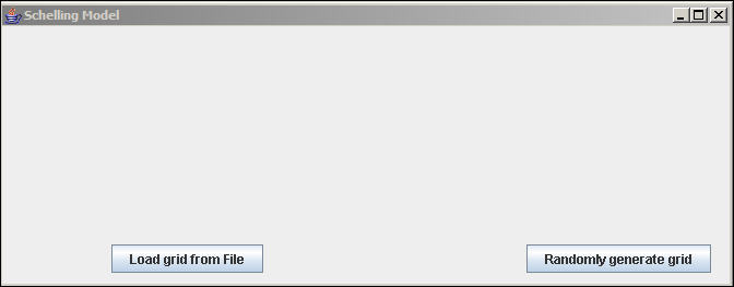
When you run the model, you will first see a screen like figure 1.
Figure 1. Opening dialog for Schelling random-movement model
You have a choice. You might want to provide your own starting configuration of reds and greens in order to explore your own particular ideas. For example, what if all the reds were initially together in a cluster in the center of the grid, and all the greens were scattered at the periphery?
If you want to input your own starting configuration, you need to prepare a plain text file called "cells.txt." We've provided an example, below, that you can download. The contents of this file looks like figure 2.
Figure 2. Example initialization file
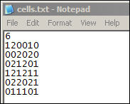
The initialization "cells.txt" file contains a single number on the first line that gives the dimension of the grid. Here, we've selected a 6 by 6 grid. The next lines show the initial values of each of the cells. A cell coded "1" is occupied by a "red" agent; a cell coded "2" is occupied by a "green" agent. And, a cell coded "0" is unoccupied.
To continue our example, though, we're going to use the second option "Randomly generate grid." When this button is selected, a dialog like figure 3 will appear.
Figure 3. Model specification for a randomly generated grid
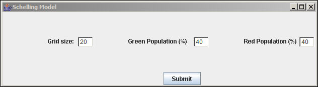
We've elected to run a model on a 20 by 20 grid, with 40% of the cells occupied by greens and 40% occupied by reds. Ask yourself: does the size of the space make any difference in the basic dynamics? does the amount of "open space" (here, 20%) make any difference? does the relative size of the two populations make any difference? (Hint, the answer is "yes" to all three questions!).
When we click on submit, we are faced with another dialog, that looks like figure 4.
Figure 4. Homophily preference specification
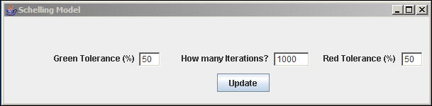
We have elected to set the "Green Tolerance" at 50%. That is, Greens will be "happy" and not want to move as long as Reds constitute no more than half of their neighbors. We've set the Red agent's tolerance to the same level. Since, in this example, there are equal numbers of Reds and Greens, this specification amounts to saying that both groups are happy with (no more than) a proportional representation of the other group in their neighborhood.
So, we have a model that is played on a 20 by 20 grid with 20% open space, and equal numbers of Red and Green actors. All actors are willing to tolerate living in mixed neighborhoods, so long as they are not a "minority." What happens when we run the model? Here we've selected only 1000 iterations -- at each iteration an actor is selected at random, it is determined whether the actor wants to move or not, and if they do want to move, they are re-located to a randomly selected open cell. Figure 5 shows a result of one run of the model with these specifications (you won't get the same exact result because of the randomizations).
Figure 5. Result of and example run
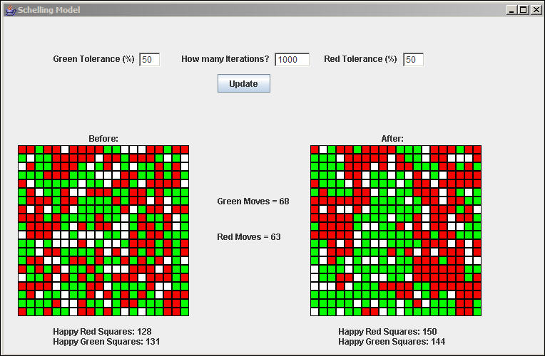
At the beginning of the simulation, 128 (of 160) Reds were in neighborhoods where they were not a minority; 131 of the 160 Green squares were.
We see that slightly more Greens moved than Reds, and that more of the members of each group (150/160 Reds and 144/160 Greens) are located in neighborhood where they are not minorities at the end of 1000 iterations.
The key finding is in the creation of homophilous residential clusters. By the end of the simulation, there is a notable tendency for separation of the reds and greens into homogeneous neighborhoods. What we have is an example of the "emergence" of a segregated pattern from the un-coordinated actions of individual agents -- none of whom has a preference to live in a segregated neighborhood!
The critical point of all of this is simple, but very important: the sum of actions by individuals may result in macro patterns that were not directed by anyone, and may not have been intended by any of the actors.
Once such a pattern emerges, however, it may come to be accepted by the actors as "normal." That is, Reds and Greens may now regard living in a neighborhood where they are the majority as "normal" and anything less as unacceptable. If this change in preference were to occur (it doesn't, in the simulation), then the pattern of separation could become an "institutionalized" "social fact."
You should download the model and experiment!
Why does this dynamic of separation happen?
What settings of model parameters (grid size, density, relative sizes of the groups, homophily preferences of the groups) might "soften" or "harden" the pattern? Are there any parameter values that will prevent segregation?
Download the executable,
source code, and configuration files (zip)
Download the executable (.jar) version
Download an example of an external initial configuration
file
In the first version of the Schelling model (above) we allowed unhappy actors to move to any open cell.
What if actors could only move from one place to another by going step-by-step, rather than leap-frogging? In a second version of the model, unhappy actors move only if they select an unoccupied cell in their own Moore neighborhood.
What effect do you think this modification will have on the dynamics?
Figure 6 shows a run of this model with the same parameter settings (but different initial conditions due to randomization).
Figure 6. Modified Schelling model with moves restricted to Moore neighborhood
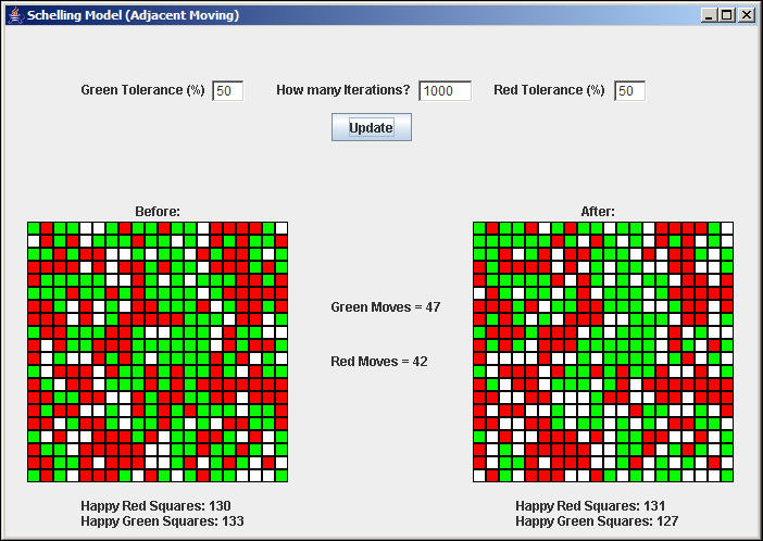
In this run (and most others) there is little net improvement -- and sometimes losses -- of "happiness" for Reds, or Greens, or both. We also note that there are fewer actual moves accomplished within the 1,000 iterations of this model, than in the less restricted model.
Do you suppose that limiting the spatial mobility of the agents will always create this result? What if the density of the population were less? What if the relative sizes of the two groups were different?
Download the executable,
source code, and configuration files (zip)
Download the executable (.jar) version
Download an example of an external initial configuration
file
Jason Martinez has provided another version of the Schelling model (written in Perl). You can download an executable version of this, or the source code. This version of the model uses the Moore neighborhood, and only local movement (that is, unhappy actors move to an available square in their local neighborhood -- not anywhere on the grid).
In this version of the model, the grid is fixed at 15 by 15 squares. The overall density is about 50%, with approximately equal numbers of Red and Blue actors.
Figure 7 shows a display of one starting configuration of the model.
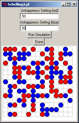
You may modify the "unhappiness" setting for the Red and Blue actors to perform experiments. In this version of the model, actors are not happy unless at least this proportion of their neighbors are of the same color. In our example, Red actors must have at least 50% Red neighbors, or they will be motivated to move; Blue actors have the same level of homphily preference.
When you click the "Run Simulation" button, the application will run 60,000 iterations in which a random actor is selected. If that actor is unhappy, they will move to a randomly chosen square in their Moore neighborhood -- if the square is unoccupied.
If a stable equilibrium is reached, the simulation stops. You can run an additional 60,000 iterations by clicking the "Run Simulation" button again.
In our example configuration, we ran the model until a stable equilibrium was reached. Figure 8 shows the result.
Figure 8. Equilibrium solution for the starting configuration and parameters in Figure 7.
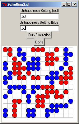
In this case, we see the emergence of a stable pattern of substantial spatial segregation of the two populations.
You should download the model and run it a number of times. Some of the things that you may want to look for are:
Download the Perl source code
Download the executable version
The Schelling agent-based model is a perfect example of "complex dynamics." There is no central director that is organizing the actors into homogeneous communities. The macro-level patterns that emerge are the natural result of individual actors following their own preferences under local circumstances -- unaware of the larger patterns that are emerging.
The Schelling model points out a process of emergent order that may be quite common in social action. Overall, and on the average in the whole population, there is no particular tendency toward segregation. But, as individual actors follow simple rules under local circumstances, local patterns emerge. Once local patterns emerge, they affect the actions of other actors, resulting (sometimes) in a "cascade" of movement. Collective action and social movements, diffusion of fads, fashion, and information, and other growth and diffusion processes may depend critically not on the attributes of the actors, but rather on the "coupling topology" or patterns of social distance among them.
The Schelling model, obviously, is not a complete or adequate theory of residential segregation (and, to be fair, Schelling never supposed that it was). But it offers some interesting insights into how unexpected patterns may emerge out of spatial interaction -- even when the actors are quite unaware, and do not intend for such outcomes. You might want to spend some time and discussion on what other kinds of phenomena might be thought of using dynamics like those of the Schelling model.
There are also some additional directions that one might want to explore in extending the basic insights of the Schelling model. To mention just a few: