Spatial Dynamics of Human Populations: Some Basic Models
Robert A. Hanneman
(robert.hanneman@ucr.edu)
Department of Sociology
University of California, Riverside
Jason Martinez
California State University
San Bernardino
Ray Holguin
CHASS College Computing
University of California, Riverside
2005
Hunting and Gathering: Predator-Prey Interactions
Most of the history of the human species (from it's origins until roughly 3,000 BC) is that of hunting-and-gathering societies. Hunting and gathering societies are generally quite small, as they derive almost all of their food by preying on other species (animal and plant), and in the process of doing so may decimate the populations of these other species. Hunting and gathering societies are also not usually spatially fixed. When the species they prey on are decimated, the human population must migrate or die off. In the case of hunting and fishing societies, the prey are also likely to migrate, and the human population must follow.
The spatial and population dynamics of hunting and gathering societies then are closely coupled with the spatial and population dynamics of the species on which they depend for food. In this page, we'll explore some of these dynamics.
We will begin with a fairly simple basic model borrowed directly from biological ecology. This model captures the population dynamics of two species -- predator and prey. In this model, prey are eaten by predators, and migrate randomly in space. Predators depend on consuming prey in order to survive. So, if prey are not plentiful, the predators must also migrate in order to find their food supply.
The basic model from biological ecology captures some key aspects of the spatial dynamics of hunting and gathering societies. Humans, at the top of the food web, are "predators" and survive by exploiting other species for food. At very low technological levels, they have little control over their food supply (i.e. they haven't yet domesticated plants or animals), and survive by hunting.
We will also modify the basic model to see if some features of human social and cultural organization may have effects on the characteristic population and spatial dynamics of predator-prey interactions: technology for storing food for short periods of time; and a tendency toward group solidarity -- which affects both the efficiency of hunting and gathering (and is practiced by many other species), as well as migration dynamics.
table of contentsThe interaction between two species in a very simple food web, where one is predator and the other prey, is a staple of biological ecology. There are many versions of predator-prey dynamics, but all are based on the interaction of two populations such that the growth rate of one population depends on the levels of population of the other. Mathematically, these are (at their core) systems of two simultaneous differential equations. Perhaps the most widely known version is the Lotka-Volterra model (Lotka, 1925, Volterra, 1926). A later version by Rosenzweig and MacArthur (1963, as reported in Turchin, 2003) is an elaboration that integrates logistic self-limitation, and non-linearity in the density/consumption relationship.
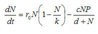
The Rosenzweig-MacArthur model can be stated in two equations, one describing the dynamics of the "prey" or "resource" population; the other describing the dynamics of the "predator" or "consumer" population. Figure 1 shows the equation for "prey."
Figure 1. Rosenzweig-MacArthur resource ("prey") dynamics
The change in the number of prey available from one time point to the next is the result of standard single-population dynamics (the first portion of the equation) and predation (the second portion, following the negative sign).
The population dynamics of the prey (resource) population, net of predation (i.e. the first portion of the equation), is a function of three interacting terms that generate a logistic relation. The "natural rate of increase" (i.e. surplus or deficit of births over deaths) r0 is the per-capita difference between births and deaths in an environment with no constraints. For human populations, estimates of this parameter usually fall in the general range of .10 -- that is, the population increases by 10% per year in the absence of any factors restraining it. Multiplying this natural rate by the current population (N) gives us the expected number of prey added per unit time, in the absence of predation and resource constraints. This number is multiplied by the term in parentheses to show how environmental resource constraints limit the natural tendency towards exponential population increase. The expected population increase is multiplied by a fraction that is one minus the ratio between the current population size and the carrying capacity (k, which is enumerated in number of prey). As N approaches k, the multiplier from density or crowding (i.e. the term in parentheses) approaches zero; as this occurs, less and less of the potential increase in population is realized. This much of the equation is a very standard self-referencing logistic growth-to-limits process.
The second term of the equation (i.e. after the minus sign) calculates the number of prey who are killed by predators (or, the number of resources used by consumers). The numerator calculates a potential number of kills; the denominator adjusts this for the density of prey to reflect the notion that the relationship between the density of prey and the number of prey killed is hyperbolic -- that is, it has an upper limit for any number of predators, regardless of how many prey are available. The numerator calculates the number of pair-wise interactions possible between prey and predators (N*P). The parameter c reflects the probability that any pair-wise interaction results in a killing (or consumption). The denominator adjusts the resulting quantity for the effects of density. As the population of prey (N) increases for any given number of predators (P), the number of prey killed per predator will increase at a decreasing rate to some upper limiting value. The speed at which this limiting value on per capita consumption is reached (i.e. satiation) is controlled by the parameter d. The greater the value of d, the lower the point of satiation.
So, although the equation looks a bit complicated, it reflects the combination of just a few basic processes: resource populations reproduce, but reproduction is limited by environmental constraints; members of the resource population are consumed at rates proportional to the number of consumers and their appetites, but this is limited by the possibility that consumers can become satiated in the presence of high densities of resources.
In the final section of this page, we'll briefly re-visit these ideas. In working with the dynamics of human populations, and varying kinds of resources, there are some modifications of the basic biological ecology theory that we might want to pursue.
The other part of the model describes the population movement of the number of predators or consumers. A version of this equation is given in figure 2.
Figure 2. Rosenzweig-MacArthur consumer ("predator") dynamics
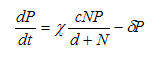
The basic logic of this equation is very similar. The population of predators or consumers increases by some rate or fraction (chi) for each unit of resources consumed. The population of predators or consumers declines exponentially at some rate (gamma) in the absence of prey or resources.
This form of the model is non-spatial. It assumes that there is homogeneous interaction within a fixed space. This is an entirely reasonable and very useful approach for many problems. Because even the basic model is a bit complicated, it is useful to first get a sense of it's characteristic behaviors without considering spatial distributions. This is what we will do in the next section. Once we have some sense of the basic dynamics, we can then begin to explore how space and connection among sub-populations may affect the results.
table of contentsThe resource-consumer (prey-predator) model is a second-order system that has a natural tendency to produce linked cyclical behavior in the levels of the two populations (for most values of most parameters). The core idea is simple: consumers use resources at rates higher than reproduction, eventually leading to collapse of the resource population. Once the resource population collapses, the consumer population must crash as well. When this happens, the resource population will eventually recover, leading to a later recovery in the consumer population, and so on. Figure 3 shows one realization of the model for a particular set of parameters.
Figure 3. One run of the resource-consumer model
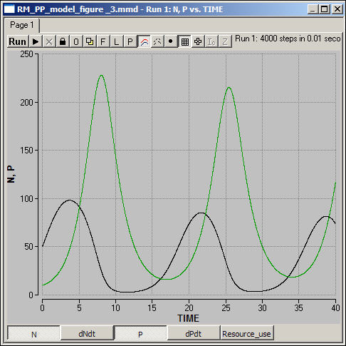
Madonna program for the resource-consumer model in figure 3.
This particular version of the model produces a "limit cycle" in which the two populations gradually approach stable (non-zero) equilibrium values. Other choices of parameters can produce population crash without recovery or cycles that do not approach an equilibrium. You might want to download the program, and experiment with different parameters to explore the range of behavior of the model.
table of contentsAs we saw above, one of the most common dynamics of the interaction between a resource and a consumer population in a single spatial area is oscillation of both populations. Among the several possible outcomes of this type, the most common is a "limit cycle" in which oscillations remain at stable amplitude, or gradually dampen to stable equilibria.
Adding a spatial dimension to this kind of dynamic can produce some additional complexity.
Let's suppose that all of our prey and predators initially occupy the central space in a 3-by-3 grid, but that they may migrate. We will suppose that a percentage of the prey who are not consumed at each cycle migrate randomly in each of the four possible directions of a von Neuman space. Predators do not migrate randomly, however. In this model, the proportion of predators who migrate is directly proportional to the rate at which predators are dying. That is, when predators are not able to find enough prey to sustain their population, some proportion of them migrate. When they migrate, they also do so randomly (that is, they engage in a random search of adjacent areas for prey).
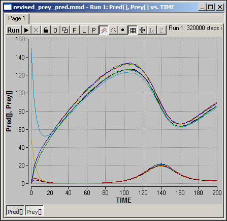
Figure 4 shows one run of this spatial model (prey populations are the upper group of lines, predator population the lower set).
Figure 4. Spatial resource-consumer model with migration (von Neuman)
Madonna code for model in figure 4
Initial values of prey or resource population for figure 4
Initial values for predators or consumers for figure 4
Initial values for carrying capacities for figure 4
The same general qualitative pattern emerges in the model with migration on a von Neuman grid. Linked cycles of the same period are established in all of the spatial areas, with slightly varying amplitudes. Try to reason the answers to these questions, and then test your intuitions by performing experiments on the system.
In the next two figures, we show some results for the same basic model with migration, but this time played in Moore neighborhoods.
Figure 5. Spatial resource-consumer model with migration (Moore): Predator dynamics
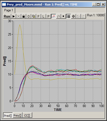
At a glance, it appears that the qualitative dynamics of this spatial model are somewhat different.
Figure 5 shows the numbers of predators or consumers in the nine spatial areas. The Moore space allows for much more rapid movement of populations over the space. Note that, where migration is more pronounced, as in this model, the severe long-term cyclical behavior of the system as a whole is so greatly dampened that it is no longer discernable. Also note that the predator populations seem to separate into three strata of final sizes.
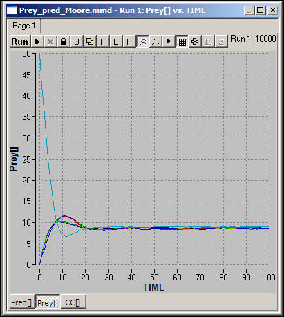
Figure 6 shows the number of prey or resources in each of the nine spatial areas under the Moore neighborhood scenario.
Figure 6. Spatial resource-consumer model with migration (Moore): Prey dynamics
Madonna code for model in figure 5 and 6
Initial values of prey or resource population for figure 5 and 6
Initial values of predator or consumer population in figure 5 and 6
Initial values for carrying capacities for figure 5 and 6
Prey cycles are not apparent as important long-run features, and all of the spatial areas have final population sizes that are very similar.
The interaction of two populations that depend on one another turns out to be a far more complicated (and, hopefully, interesting) problem than one might have first thought. In the case where one population "preys" on the other, a common dynamic is one of linked cyclical rise and fall in both populations.
We've been pretty abstract in our discussion, not linking this kind of model to sociological problems. But, to make this more "sociologically real," think about these three cases:
a) Suppose that we were describing the dynamics of the population of a hunting or fishing society -- plains Indians and Buffalo or Eskimos and seals.
b) Suppose that the "resources" or "prey" were renewable natural resources -- like grains, nuts, and berries; and the human population derived most of their sustenance from gathering.
c) Suppose that the "resources" or "prey" were the population of peasant producers in an agricultural society, and that the "predators" were landlords and the state/church.
d) Suppose that the "resources" were workers, and that the "consumers" were capitalists.
One should not, probably, draw over-simple analogies between biological "predators" and "prey" and human social dynamics. As you think about each of the cases, also think of why the models we've developed here probably don't exactly describe human systems. Then, think through how you might modify these models to make them more realistic and useful for studying non-human/human or human/human systems.
One very important set of alternative approaches to two-population interactions specify different kinds of relations between the two populations. What if the two populations preyed on one another, rather than one exploiting the other? What if the two populations depended on each other for survival (as in parasite host dynamics?).
What if there were more than two types of populations, and a more elaborate "food web" connecting them (e.g. Turchin's model of peasant producers, exploiting landlords, and a state apparatus that taxes the landlords)? What is some populations could migrate, but others could not? There are many interesting questions (and questions that may seem more sociologically realistic) that one can explore beginning with the very simple models developed here.
In the cases we've looked at hear, explicit treatment of space has suggested that some rather different kinds of dynamics can result than in with a single spatial area. In our cases, migration has acted as something of a "safety valve" that dampens or even eliminates the inherent tendency of the predator-prey model toward boom-and-bust cycles. Different choices about the connective topology among spatial areas, and different rules about migration, however, would not necessarily produce the same kinds of results.
table of contents