Spatial
Dynamics of Human Populations: Some Basic Models
Robert A. Hanneman
(robert.hanneman@ucr.edu)
Department of Sociology
University of California, Riverside
Ray Holguin
CHASS College Computing
University of California, Riverside
Jason Martinez
California State University
San Bernardino
2005
An Estonian translation has
kindly been made available by Paula-Maria Niculescu:
http://www.bildelarstore.se/science/sundimus-suremus-kandevoime-ja-migratsiooni
Fertility,
Mortality, Carrying Capacity, and Migration
Virtually all sociological
theories regard the number of actors in populations to be a critical cause and
effect of other important things. For example, large numbers of
individual persons need to be concentrated before a complex division of labor
can emerge; a high level of differentiation can provide productivity gains that
allow expansion of population. Population dynamics are a central part of
theories of small groups, communities, informal and formal organizations, whole
societies, and the global system. Models of population dynamics are quite
advanced in human demography and ecology. Many of the insights of these
literatures have been applied to other types of populations of social agents
(organizations, societies, etc.).
On this page, we are going to
develop a very simple model of population dynamics. We begin with
Malthus' (and many others) insight that the numbers in populations tend to
increase exponentially in the absence of any environmental limits. Of
course, populations of social agents do not reside in limitless
environments. So, we will next add the idea of "carrying
capacity," and model how it limits population growth. Taken together,
these dual forces of growth and limitation make up the classical
"logistic" population growth model that is the starting point for
almost all demographic/ecological models.
Populations also exist in
space, and individuals may migrate from one place to another. The last
part of our basic model development will explore some of the implications of
movements of individuals from one population to adjacent populations. We
will examine one very simple theory of migration (there is a large and rich literature
of theory and empirical research on this subject). In our model, there is
a normal tendency for some members of one population to migrate to adjacent
populations. When the resources of an area are large (i.e. the carrying
capacity is high) relative to the size of the population, however, individuals
will be less likely to migrate. When resources are tight (i.e. population
exceeds carrying capacity), the natural tendency for migration is
accelerated. We are going to suppose that the retardation and acceleration
of migration based on resource availability are exponential; that is, small
deviations of population from carrying capacity have little effect on normal
migration, but larger deviations have much greater effects.
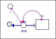
Figure 1 is a systems
dynamics diagram of a very simple population model. The number of agents
in the population at any instant is "N." "N" can
increase or decrease (indicated by the double-headed "flow") and is
the accumulation of changes in population that occur over time (dN/dt).
Figure 1. Population growth in an
unlimited environment: Model
The causal theory is really
about what causes population to be increasing or decreasing over time; that is,
what causes dN/dt.
The actual level of population is simply the accumulation of all past changes.
In our very simple
demographic model, we suppose that, in the absence of any limits, there will be
a net change in population (r = a surplus of births over deaths, or a surplus
of deaths over births) that can be expressed as a probability. If
"r" is a positive number, for example, .05, then there is a 5% chance
that each individual in the population will produce one more off-spring in one
unit of time than the number of deaths in that interval. The total net
number of off-spring produced, then, is r*N (the probability of any individual
reproducing above the death rate, times the
number of individuals). Depending on the kinds of entities being modeled,
different choices of "r" would be made. We'll suppose that we
are examining populations of individual humans, and we'll choose a value of
"r" between zero and one.
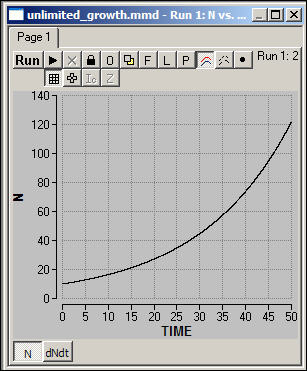
What will happen to the size
of the population when we observe this process acting over time? Figure 2
shows a simulation of the model dN/dt = r*N, for an initial value of N=10, and r = .05.
Figure 2: Population
growth in an unlimited environment: Simulation
download the Madonna model for Figure 2
The size of the population
increases at an increasing rate. Even though the risk that any one agent
has an off-spring in excess of the death rate in any one period of time is a
constant, the size of the population "at risk" is steadily
increasing. The total population, therefore, increases exponentially
without limit.
Social agents, however, do
not live in unlimited resource environments. At any one time and place,
there are limits to how many individuals can be supported by the resources
available. The maximum number of agents that can be supported (at some
defined level, usually "subsistence") is the "carrying
capacity." Figure 3 modifies our theory to include the carrying
capacity ("k") as an additional cause of over-time change in the rate
of change of population.
Figure 3. Logistic net population growth:
Model
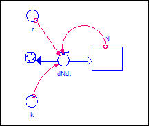
One might imagine a number of
ways that carrying capacity affects the net reproduction rate. It may be
that when population exceeds the carrying capacity the death rate is increased;
it may be that as population grows large relative to the death rate, there is a
restriction in fertility. For our model, we are going to use this
equation to describe the relationship:
dN/dt = (r*N) * (1 - (N/k))
The first part of this is
familiar -- it is our exponential growth model. The second part describes
how carrying capacity restricts population growth. As population
approaches carrying capacity (that is as N/k gets closer to one), the
right-hand part of the expression becomes closer to zero. As this happens, less and less of the tendency toward exponential
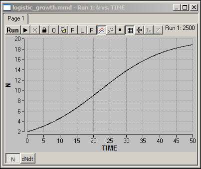
growth is "realized." Figure 4 shows a simulation of
this version of the model.
Figure 4. Madonna logistic model:
Simulation
download the Madonna model for Figure 4
When population is low, it
tends to increase at an increasing rate. Beyond a turning point or
threshold, however, the growth rate becomes less and less as the carrying
capacity is approached. The result is a smooth "S-shaped" curve
called the "logistic" growth curve.
There are many more complex
models of basic population dynamics than the simple one we've developed.
Since our main concern is with the effects of spatial coupling of populations in
making for complex population dynamics, we're not going to explore these issues
here.
Suppose that we had more than
one population, and that the populations were adjacent. Furthermore,
suppose that individuals could migrate from one population to the other.
Figure 5 shows a systems dynamics diagram of two populations
"coupled" by bi-directional migration.
Figure 5. Two-region model with migration
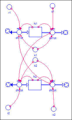
There is a basic logistic
demographic model operating in each population (N1 and N2). This time,
however, we've shown an additional source of change in each population - dMdt. This is the rate of migration out of each
population. We also show arrows connecting the out-migration from each
population to the growth rate in the other. This indicates that agents
who leave one population are migrating to the other.
Now, we need a theory of
migration to determine how many individuals will move from one region to the
other. There are many sophisticated theories, and we will develop only a
very simple one here. We will suppose that some fraction of the
population of each area will migrate in each period of time, all else
constant. This fraction is indicated as "c" in Figure 5.
So, the number of persons leaving each population as a result of this
"normal" or "frictional" movement is dM/dt = c * N.
When resources are plentiful
in a region (i.e. population is less than carrying capacity, N/k < 1) we
suppose that "normal" migration is reduced. When there is
scarcity (i.e. population is greater than carrying capacity, N/k > 1), we
suppose that "normal" migration is amplified: dM/dt = (c * N) * (N/k). We
suppose, however, that the effect of wealth or scarcity on the propensity to
migrate is not linear. Small differences of population from carrying
capacity do not have much impact on migration, as the motivation to move (or
stay) are not strong enough to overcome the "transaction costs" and
"uncertainty" involved in moving. However, as conditions become
more extreme (either much greater wealth per capita, or much greater scarcity),
we suppose that the response (either the commitment to stay, or the motivation
to leave) become stronger at an increasing rate. We model this by
supposing that the effect of N/k on normal migration is in the form of an
exponential (in our simple example, we use (N/k)2.
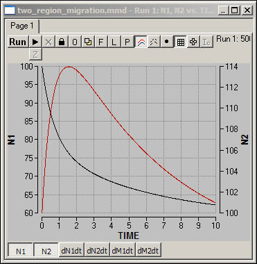
Figure 6 shows one simulation
of the two-region model in which the population in region N1 (blue) is
initially higher than carrying capacity, and the population in region N2 (red)
is initially at carrying capacity.
Figure 6. Simulation of two-region model
with migration
download the Madonna
model for Figure 6
Since there is
"excess" population in the blue region (N1), there is rapid net
migration, initially from N1 to N2. Since the red region (N2) is already
at capacity, it's population is swelled by new
immigrants, but then declines as mortality exceeds fertility. As the
model runs, the population of both regions approaches their carrying
capacities, and migration rates come closer and closer to "normal."
You might want to download
the program and conduct some experiments. The main factors underlying the
dynamics in this model are the sizes of the initial populations, and how far
these populations are from carrying capacity. To get a good grasp on the
range of behavior that the theory can predict, you might design a set of
experiments:
- What if
both regions are above carrying capacity?
- What if
both regions are below carrying capacity?
- What if
one is above and the other below carrying capacity?
- Do the
patterns observed in the three situations above hold true when the
populations and carrying capacities of the regions are different from one
another and when the regions are the same?
Now that we have the basic
ideas, we want to expand the model to include some greater spatial
complexity.
There are a number of issues
that we could explore. Here are a couple interesting ones that we won't
examine; but you're invited to download the model and experiment.
The size of the space, and how boundaries are treated is consequential for
dynamics. For our examples, below, we will look at a very simple 3-by-3
space. In our model, agents migrate from each space to all available
Moore neighbors. So, "corner" squares have 3 neighbors, edge
squares have 5, and central squares have 8. In our model, the total number of migrants are divided among the available
neighbors. One might, alternatively, chose proportions migrating to each
neighbor randomly, or choose a single neighbor and have all migrants move in
that direction.
The "coupling
topology" (e.g. is migration done in neighborhoods, along a network, or
over continuous distances) of the populations is an interesting area to
explore. We'll use the Moore neighborhood approach to space. A Von Neuman, social network distance, or spatial gradient
approach would produce different results.
The two questions we would
like to explore, briefly, are what happens when population is not in spatial
equilibrium, and what are the effects of non-homogeneous distributions of
carrying capacity across space?
Non-homogeneous
initial population distribution
Populations often first
appear at a single point in a space, and "disperse" by migration
throughout the space. In Figure 7, we've done one experiment with our
simple model to try to get a sense of what the spatial dynamics of population
dispersion look like.
In the current scenario, we
begin with all population concentrated in the central square of a 3-by-3
grid. All the squares on the grid have equal carrying capacity of 1,000
individuals, and the size of the population in the central square, initially,
exceeds this carrying capacity (1,500). Figure 7 shows the results of a
simulation of these initial conditions.
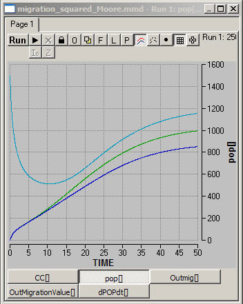
Figure 7. population
movements in 9 square grid, empty except for 1.5 times capacity in center
download the
Madonna model for Figure 7
download the initial population data file for Figure 7
download the carrying capacity data file for Figure 7
The top, light blue, line
shows the population trend for the central location. Since the population
there exceeds carrying capacity, there is a lot of out-migration
initially. After a time, out-migration slows as population size declines
below carrying capacity; some return migration begins to occur; and internal
logistic population growth eventually comes to dominate the dynamics.
Note, however, that the apparent equilibrium population of the central square
seems to exceed it's
carrying capacity.
The non-central populations
are either edges or corners, and we see that the shape of
their trends (the green and dark blue lines) are similar, but that the
final equilibrium values are not.
Some questions to think
about:
- Why does
the system reach an equilibrium?
- Why is the
equilibrium level of population the same in all spatial areas? After
all, the carrying capacity of all the areas is the same.
- When the
system has reached equilibrium, does this mean that there is no longer any
migration occurring?
- Why does the first part of the curves look exponential, and
the later part of the curves look logistic? Can you think of
different initial conditions that would produce different looking trends?
- Where
would you prefer to live? Where is the level of per capita living
highest?
- What would
the patterns look like if the grid were much larger?
- What would
the patterns look like if the initial population was located in a corner,
instead of the center?
A key lesson here is that
space matters. Even though the birth-death-migration model and it's parameters are identical in all spaces, and even though
the carrying capacity of the environment is the same in all spatial areas, the
"equilibrium" levels of population are not.
Non-homogeneous
carrying capacity
Let's consider an alternative
scenario where population densities are equal, but
carrying capacities are not. Imagine that we moved 1,000 people to each
of the 9 grid squares. But suppose that only two corner squares had the
capacities to support any significant populations. What will
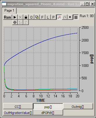
happen? Figure 8 shows one scenario like this.
Figure 8. All cells at 1000 population,
carrying capacity at 5000 in two corners, 10 elsewhere
download the
Madonna model for Figure 8
download the initial population data for Figure 8
download the carrying capacity data for Figure 8
What happens, of course, is
that people living in squares that have low carrying capacity are going to move
out, looking for spaces where the level of living is higher. Within just
a few time steps, the "poor" areas have nearly emptied of population,
and population has become concentrated in the two "rich" areas.
From that point on, logistic growth dominates the dynamics in all regions (but
operates at very different levels).
You might want to download
this program and experiment with creating a larger grid that is a
"map" of the levels of resources available across some real
geographical space. What will the equilibrium result for the distribution
of population look like?
Directions
for development of more sociologically realistic models
The core ideas of the very
simple model here are common across a wide range of sociological
theories. The general idea that the spatial distribution and
concentration of populations of social agents (people, families, organizations,
etc.) depend on net reproduction and migration occurring on a "sub-strate" of carrying capacity is a starting point
shared by most theories of social dynamics.
Demographic theory has
explored in great detail the relationships of fertility and mortality to
carrying capacity (and to other factors, such as distributional
inequality). Human ecology has explored in great detail the relationships
between carrying capacity, population, and migration. More sophisticated
treatments of these connections within the spatial framework would be useful
directions for future work.
Classical sociological theory
also suggests a number of directions for future work that would make the basic
model more realistic -- as well as making it a bit more dynamic and complex.
Social
organization increases carrying capacity
In the model developed here,
"carrying capacity" is treated as a constant. There are a
number of problems with this simplification, and these problems provide
opportunities for further work:
The carrying capacity of an
area may consist of both renewable and non-renewable resources.
Non-renewable resources must be replaced with substitutable resources (or made
irrelevant to survival by technological change), and "carrying
capacity" declines as the levels of these resources decline.
Renewable resources are not consumed at constant rates. Rates of
consumption depend on distributional equality, marginal costs of production,
and the speed with which resources reproduce. In many cases, over-use of
renewable resources may drive the resources to extinction, resulting in a
permanent loss of carrying capacity.
Very importantly, the
carrying capacity of spaces for human populations depends very much on the
technology available. The carrying capacity of resource environments can
be hugely expanded by the application of technology -- new materials become
resources as we learn how to exploit them, and the efficiency of use of
resources can be greatly modified by improved technology. The
relationship between population density and level of technological development
is an are of considerable
theoretical and empirical interest and controversy. Making "carrying
capacity" endogeneous to the model has many
interesting theoretical possibilities.
Social
organization drives systems beyond sustainable limits
As population increases and
concentrates, the division of labor increases, increasing productivity and
carrying capacity. However, this process is ultimately bounded by the
physical environment and the level of technological knowledge. The higher
productivity of complex social organization depends on increasingly large
investment in infrastructure and coordinative activity. It may be,
however, that there are decreasing marginal returns
in productivity to increased social complexity.
The increasing division of
labor and growth of the coordinative component of social structures also
re-distributes power in ways that make tendencies toward growth in the
coordinative component self-generating. Many theorists have held that
societies may escape collapse for lengthy periods of time by increasing the
complexity of organizational coordination; ultimately, however, productivity
does not expand at the same rate as overhead, and complex social structures may
collapse. Adding theories of the division of labor and it's consequences to the current model would enable us to
add a spatial dimension to macro sociological theories of growth and collapse
that is (largely) missing in current work.
A key aspect of the
consequences of population growth and increasing division of labor in society
is the emergence of class structures that unequally distribute resources.
The response functions of births, deaths, migration, and carrying capacity may
be greatly affected by levels of social inequality.
In spatial models like the
one here, there is a second form of social inequality that is likely to be very
consequential -- inequality between populations. Differing levels of
carrying capacity across space act as powerful "pull" factors in
migration. Our current model treats only the "push" side of the
equation. The simple gravity model developed on another page in this
website might be further developed as a way to add "pull" or
"attraction" between populations to the model.
index of the spatial models website