6. Working with network data
This chapter is about the kinds of "data structures" that network analysts work with most frequently, and some of the most common kinds of transformations and manipulations of these structures.
Data Structures
Most everyone reading this is very familiar with the kind of "data structure" that is used in many statistical studies. The rectangular array of data that we are used to seeing in SPSS, SAS, Excel, and other programs is a "structure" that is defined by its rows (which represent cases) and columns (which represent variables). An example is shown as figure 6.1.
Figure 6.1. Rectangular data array
| ID | Sex | Age | Married |
| Bob | M | 42 | 1 |
| Carol | F | 44 | 1 |
| Ted | M | 39 | 0 |
| Alice | F | 27 | 0 |
Earlier, we emphasized that the social network perspective leads us to focus our attention on the relations between actors, more than on the attributes of actors. This approach often results in data that have a different "structure" in which both rows and columns refer to the same actors, and the cells report information on one variable that describes variation (in the case of the example below, simple presence of absence of a tie) in the relations between each pair of actors. An example is given as figure 6.2.
Figure 6.2. Square data structure for social network data
| Friendship ties | ||||
| Bob | Carol | Ted | Alice | |
| Bob | --- | 1 | 0 | 0 |
| Carol | 0 | --- | 1 | 0 |
| Ted | 1 | 1 | --- | 1 |
| Alice | 0 | 0 | 1 | --- |
A "data structure" is simply the way in which information is recorded. These two examples are both two-dimensional (rows and columns). It is possible, for a data structure or data object to have more than two dimensions. For example, if we wanted to also record information about the network relations of who is married to whom, we would usually create another table of actors by actors (that is, the row and column indexes would be the same), and record the presence or absence of marital ties. If we "stacked" the two tables together, we would have a 4 by 4 by 2 "data structure." Counts of the rows, columns, and matrices (or "slices") do not include the labeling or indexing information (i.e. it's not 5 x 5 x 3).
Social network analysis data structures:
Network analysts work with a variety of data structures. In this chapter, we'll look tools for creating and manipulating the most common types.
One major "type" of data structure is the actor-by-actor matrix (like the friendship data above). This kind of structure is, by definition, a "two-dimensional," and "square" (the number of rows and columns are equal). The information in each cell provides information about the relation between a particular pair of actors.
The two-dimensional actor-by-actor matrix is very often expanded into a "third dimension" by adding "slices" that represent additional kinds of relations among the actors. For example, we might have an actor-by-actor matrix of Bob, Carol, Ted, and Alice that records the degree of "liking" directed from each to each. In addition, we might add a second "slice" that records the presence or absence of a kinship relation between each pair. These kinds of 3-dimesional network data structures are "multi-plex." That is, they represent multiple relations among the same sets of actors. Some of the special issues in working with multi-plex data are discussed in chapter 15.
The other major "type" of data structure that network analysts use looks a lot like the "rectangular data array" from conventional statistical work. The data structure consists of rows (representing actors) by columns (representing attributes of each actor -- what would be called "variables" in statistics). Such an array might record just one attribute, in which case the data structure would be a "column vector." Or, such an array might record a number of attributes of each actor. Network analysts think of this kind of "rectangular" array of actors by attributes simply as a collection of vectors.
The "rectangular" data structure (called an "attribute" data set) is used in a number of ways in network analysis.
The "rectangular" data structure can also be used to record information about the relationships between two types of nodes (called bi-partite data). This use is so common and so important that it has a special name -- and "incidence" or an "affiliation" matrix. For example, the rows might be indexed by actors (e.g. Bob, Carol...); but, the columns might be the organizations that employ the actors (IBM, Sun, Microsoft...). Entries in the cells indicate the presence or strength of the relation between an actor and an employer.
Incidence or affiliation data is particularly important in many social network analyses because it is "multi-level." Actors may be tied together because they are present in the same place, time, or category (that is, they are in the same "incident" to, or are "affiliated" with the same structure). But such data also show how "incidents" are tied together by the "co-presence" of actors. Incidence data involving two kinds of actors (bi-partite) data are very important in network analysis because they are often our best window into questions of "agency and structure" or "macro-micro linkages."
In this chapter we will describe some of the most common kinds of manipulations that social network analysts use in creating data structures, and changing their structures to meet the needs of particular research questions. Even though this chapter is going to be a bit long, it hardly covers all the possibilities. Different questions require different data structures. The examples and tools here will get you started.
table of contentsUCINET datasets are stored in a special (Pascal) format, but can be created and manipulated using both UCINET's and other software tools (text editors and spreadsheets). Each UCINET dataset consists of two separate files that contain header information (e.g. myfile.##h) and the data lines (e.g. myfile.##d). Because of this somewhat unusual way of storing data, it is best to create data sets with the internal spreadsheet editor or DL language tools, or to import text or spreadsheet files and save the results as UCINET files.
There are several ways of creating data files that UCINET can read.
The spreadsheet editor. UCINET has a built-in spreadsheet editor that can be used to enter case and variable labels and data values (data>Spreadsheets>matrix). This editor allows you to specify the number of rows and columns, and has the nice feature of being able to specify that a data set is symmetric. If we are recording a data set where ties among actors are not directed, this feature saves half the data entry. There are also tools to fill the matrix with zeros (a common starting point for many data sets that have sparse connections among actors), permuting rows, symmetrizing and dichotomizing (see discussions in the sections below), and copying row labels to the column labels (if the data are symmetric, you need only enter the labels once).
The UCINET spreadsheet editor can import and export Excel spreadsheets, so you can use tools in both programs to full advantage. To import Excel to UCINET, be sure to save your spreadsheet as version 4 or earlier; the multi-sheet format of more recent Excel versions isn't supported in UCINET.
If you have a fairly small dataset, the UCINET spreadsheet editor is a good choice for making single matrix datasets, which are automatically saved as UCINET files that can be used by other parts of the program.
Importing (and Exporting). Data sets can be moved from a number of other program's data file formats into UCINET's. The Data>Import>... menu item supports import from NetDraw (VNA format), Pajek, Krackplot, and Negopy. It also supports importing raw ASCII text files, and files saved as Excel spreadsheets (version 4 or earlier). So, if you started with a NetDraw drawing, for example, and saved the results as VNA, you may import this into UCINET for calculating network measures. I'm more comfortable with Excel than with UCINET's editor, so I usually make data sets in Excel, and import them.
When UCINET imports a file, it will produce a window with your results. Check to make sure they are correct! When the import is performed, UCINET automatically saves the data files in UCINET format in the default directory.
It's often a good idea to set up a new directory for each project, and to set the default to this new directory using the file-cabinet icon on the toolbar, or File>Change default folder.
UCINET datasets can also be exported for use in other programs. Data>Export>... will produce Excel, raw ASCII text, Pajek, Mage, Metis, and Krackplot files.
The DL language: If you've been looking at the UCINET Data menu as you read the preceding discussion, you may have noted that the program imports and exports "DL" files. DL (for "data language") is a very powerful and (fairly) simple language that allows the creation of quite complex and large UCINET data sets with minimal data entry.
DL language files are plain ASCII text files that can be created with any editor (be sure to store the results as plain text). A quite complete reference guide is provided in UCINET (Help>Help Topics>DL).
The DL language can be a bit picky, and it does take a little effort to figure out how to do exactly what you want to do with it. But, there are a number of circumstances where it is well worth the effort -- when compared to using a spreadsheet. Particularly, if your data set consists of multiple matrices, and if the data are fairly sparse, or if the data set has many rows and columns; then the DL file is the right way to go.
We won't explore the language in any detail here -- the help file is quite good. Figure 6.3 shows an example of a DL file that illustrates a few of the features.
Figure 6.3. Example DL language file
dl
n=9, format=edgelist1
labels:
A,B,C,D,E,F,G,H,I
data:
1 1
1
1 2
1
1 6
1
.
.
.
8 7
1
9 9
1
The file begins with "dl" to indicate file type, and specification of the dimension of the data structure (the language allows specification of number of rows, columns, and matrices). Labels for the nodes are given in the "labels:" paragraph. The data are given in a "data:" paragraph.
The interesting thing in this example is the use of the format=edgelist1 command. This tells UCINET to read the data lines in a way that is very efficient. The edgelist1 format is a set of rows, each one of which identifies two nodes and the value of the connection between them. In the resulting data set, all entries are zero, except those that have been specified. So, among our nine actors, there is a tie from actor 1 to actor 1, a tie from actor 1 to actor 2, a tie from actor 1 to actor 6, etc. Here, the matrix is binary -- the value of each tie (the third entry on each line) is 1.
Another very useful format= method is nodelist1. In this format, each line of data consists of the name (or number) of an origin node, followed by all of the nodes to which it has a connection (this particularly format is for zero/one data on the presence or absence of a connection). This approach then requires only one line of data for each actor. For example, a line in the data: section that read: 3 5 6 19 24 would indicate that actor number 3 had a binary directed tie to actors 5, 6, 19, and 24.
These, and other methods available in DL allow the entry of very large and complex data sets with the greatest efficiency and minimum typing. If you are facing a problem with many cases, connections, or kinds of connections, invest a little time in DL.
It is not at all unusual for the analyst to want to change the values that describe the relations between actors, or the values that describe the attributes of actors. Suppose the attribute "gender" had been entered into a data set using the values "1" and "2," and we wanted to change the attribute to be "Female" coded as "0" and "1." Or, suppose that we had recorded the strength of ties between companies by counting the number of members of boards of directors that they had in common. But we then decide that we are only interested in whether there are members in common or not. We need to change the coded values to be equal to "0" if there are no board members in common, and "1" if there are any (regardless of how many).
Just like statistical packages, UCINET has built-in tools that do some of the most common data transformations.
Transform>Recode is a very flexible and general purpose tool for recoding values in any UCINET data structure. its dialog box has two tabs: "Files" and "Recode."
In the files tab, you can browse for an input dataset, select which matrices in the set to recode (if there is more than one), which rows and columns to recode (this is good if you are working on a collection of attribute vectors, for example, and only want to recode selected ones), whether to recode the values on the diagonal, and the name of the output dataset.
In the recode tab, you specify what you want done by creating rules. For example, if I wanted to recode all values 1, 2, and 3 to be zero; and any values of 4, 5, and 6 to be one, I would create to rules. "Values from 1 to 3 are recoded as 0" "Values from 4 to 6 are recoded as one." The rules are created by using simple built-in tools.
Almost any transformation in a data set of any complexity can be done with this tool. But, often there are simpler ways to do certain tasks.
Transform>Reverse recodes the values of selected rows, columns, and matrices so that the highest value is now the lowest, the lowest is now the highest, and all other values are linearly transformed. For example, the vector: 1 3 3 5 6 would become the vector 6 4 4 2 1.
If we've coded a relationship as "strength of tie" but want our results to be about "weakness of tie" a "reverse" transform would be helpful.
A common task in network analysis is to calculate the "similarity" or "distance" between two actors based on their relationships with other actors (more on this in the sections on equivalence, later). "Similarity" scores can be "reversed" to become "dis-similarity;" "distance" scores can be "reversed" to be "nearness" scores with this tool.
Transform>Dichotomize is a tool that is useful for turning valued data into binary data. That is, if we have measured the strength of ties among actors (e.g. on a scale from 0 = no tie to 5 = strong tie), the "dichotomize" can be used to turn this into data that represent only the absence or presence of a tie (e.g. zero or one).
Why would one ever want to do this? To convert an ordinal or interval measure of relation strength into simple presence/absence may throw away considerable amounts of information. Many of the tools of social network analysis were developed for use with binary data only, and give misleading results (or none at all!) when applied to valued data. Many of the tools in UCINET that are designed for binary data will arbitrarily dichotomize interval or ordinal data in ways that might not be appropriate for your problem.
So, if your data are valued, but the tool you want to use requires binary data, you can turn your data into zero-one form by selecting a cut-off value (you will also have to select a "cut-off operator" and decide what to do with the diagonal.
Suppose, for example, I'd measured tie strength on a scale from 0 to 3. I'd like to have the values 0 and 1 treated as "0" and the values 2 and 3 treated as "1." I would select "greater than" as the cut-off operator, and select a cut-off value of "2." The result would be a binary matrix of zeros (when the original scores were 0 or 1) and ones (when the original scores were 2 or 3).
This tool can be particularly helpful when examining the values of many network measures. For example, the shortest distance between two actors ("geodesic distance") might be computed and saved in a file. We might then want to look at a map or image of the data at various levels of distance -- first, only display actors who are adjacent (distance = 1), then actors who are one or two steps apart, etc. The "dichotomize" tool could be used to create the necessary matrices.
Transform>Diagonal lets you modify the values of the ties of actors with themselves, or the "main diagonal" of square network data sets. The dialog box for this tool allows you to specify either a single value that is to be entered for all the cells on the diagonal; or, a list of (comma separated) values for each of the diagonal cells (from actor one through the last listed actor).
For many network analyses, the values on the main diagonal are not very meaningful, and you may wish to set them all to zero or to one -- which are pretty common approaches. Many of the tools for calculating network measures in UCINET will automatically ignore the main diagonal, or ask you whether to include it or not.
On some occasions, though, you may wish to be sure that ties of an actor with themselves are treated as present (e.g. set diagonal values to 1), or treated as absent (e.g. set diagonal values to zero).
Transform>Symmetrize is a tool that is used to turn "directed" or "asymmetric" network data into "un-directed" or "symmetric" data.
Many of the measures of network properties computed by UCINET are defined only for symmetric data (see the help screens for information about this). If you ask to calculate a measure that is defined for only symmetric data, but your data are not symmetric, UCINET either will refuse to calculate a measure, or will symmetrize the data for you.
But, there are a number of ways to symmetrize data, and you need to be sure that you choose an approach that makes sense for your particular problem. The choices that are available in the Transform>Symmetrize tool are:
>Maximum looks at each cell in the upper part of the matrix and the corresponding cell in the lower part of the matrix (e.g. cell 2, 5 is compared to cell 5, 2), and enters the larger of the values found into both cells (e.g. 2, 5 and 5, 2 will now have the same output value). For example, suppose that we felt that the strength of the tie between actor A and actor B was best represented as being the strongest of the ties between them (either A's tie to B, or B's tie to A, whichever was strongest).
>Minimum characterizes the strength of the symmetric tie between A and B as being the weaker of the ties AB or BA. This corresponds to the "weakest link," and is a pretty common choice.
>Average characterizes the strength of the symmetric tie between A and B as the simple average of the ties AB and BA. Honestly, I have trouble thinking of a case where this approach makes a lot of sense for social relations.
>Sum characterizes the strength of the symmetric tie between A and B as the sum of AB and BA. This does make some sense -- that all the tie strength be included, regardless of direction.
>Difference characterizes the strength of the symmetric tie between A and B as |AB - BA|. So, relationships that are completely reciprocal end up with a value of zero; those what are completely asymmetric end up with a value equal to the stronger relation.
>Product characterizes the strength of the symmetric relation between A and B as the product of AB and BA. If reciprocity is necessary for us to regard a relationship as being "strong" then either "sum" or "product" might be a logical approach to symmetrizing.
>Division characterizes the strength of the symmetric relation between A and B as AB/BA. This approach "penalizes" relations that are equally reciprocated, and "rewards" relations that are strong in one direction, but not the other.
>Lower Half or >Upper
Half uses the values in one half of the matrix for the other
half. For example, the value of BA is set equal to whatever AB is.
This transformation, though it may seem odd at first, is quite helpful. If
we are interested in focusing on the network properties of
"senders" we would choose to set the lower half equal to the upper
half (i.e. select Upper Half). If we were interested in the structure of
tie receiving, we would set the upper half equal to the lower.
>Upper > Lower or >Upper < Lower (and similar functions available in the dialog box) compare the values in cell AB and BA, and return one or the other based on the test function. If, for example, we had selected Upper > Lower and AB = 3 and BA = 5, the function would select the value "5," because the upper value (AB) was not greater than the lower value (BA).
Transform>Normalize provides a number of tools for rescaling the scores in rows, in columns, or in both dimensions of a matrix of valued relations. A simple example might be helpful.
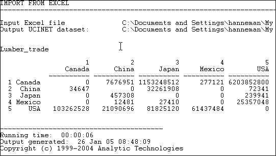
Figure 6.4 shows some data (from the United Nations Commodity Trade database) on trade flows, valued in dollars, of softwood lumber among 5 major Pacific Rim nations at c. 2000.
Figure 6.4. Value of softwood lumber exports among five nations
Suppose we were interested in exploring the structure of export partner dependence -- the disadvantage that a nation might face in establishing high prices when it has few alternative places to sell its products. For this purpose, we might choose to "normalize" the data by expressing it as row percentages. That is, what proportion of Canada's exports went to China, Japan, etc. Using the row normalization routine, we produce figure 6.5.
Figure 6.5. Row (sending or export) normalized lumber trade data
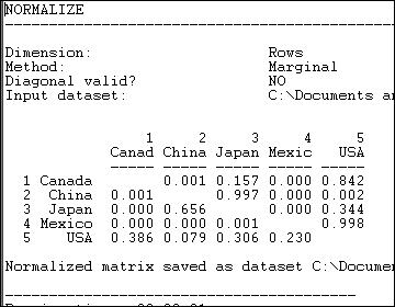
Graphing the original trade-flow data would answer our question, but graphing the row normalized data gives us a much clearer picture of export dependency. If we were interested in import partner trading concentration, we might normalize the data by columns, producing figure 6.6.
Figure 6.6. Column (receiving or import) normalized lumber trade data

We see, for example, that all of Canada's imports are from the USA, and that virtually all of the USA's imports are from Canada.
The >Transform>Normalize tool provides a number of ways of re-scaling the data that are frequently used.
Normalization may be applied to either rows or columns (as in our examples, above), or it may be applied to the entire matrix (for example, rescaling all trade flows as percentages of the total amount of trade flow in the whole matrix). Normalization may also be applied to both rows and columns, iteratively. For example, if we wanted an "average" number to put in each cell of the trade flow matrix, so that both the rows and the columns summed to 100%, we could apply the iterative row and column approach. This is sometimes used when we want to give "equal weight" to each node, and to take into account both outflow (row) and inflow (column) structure.
There are a number of alternative, commonly used, approaches to how to rescale the data. Our examples use the "marginal" total (row or column) and set the sum of the entries in each row (or column) to equal 1.0. Alternatively, we might want to express each entry relative to the mean score (e.g. divide each element of the row by the average of the elements in a row). Alternatively, one might rescale by dividing by the standard deviation, or both mean and standard deviation (i.e. express the elements as Z scores). UCINET supports all of these as built-in functions. In addition, scores can be normalized by Euclidean norm, or by expressing each element as a percentage of the maximum element in a row.
Rescaling transforms like these can be very, very helpful in highlighting structural features of the data. But, obviously different normalizing approaches highlight very different features. Try thinking through how what applying each of the available transformations would tell you for some data that describe a relation that you are interested in. Some of the transformations will be completely useless; some may give you some new ideas.
table of contentsBecause UCINET data files are stored in a somewhat unusual dual-file format, it is usually most convenient to do basic file-handling tasks within UCINET.The program has basic file handling tools within it. Using these has the advantage of automatically dealing with both the .##h and .##d files that make up each UCINET dataset. If you use file handling commands outside UCINET (e.g. using Windows), you need to remember to deal with both files for each data set.
File utilities:
File>Copy UCINET Dataset
File>Rename UCINET Dataset
File>Delete UCINET Dataset
These commands do exactly what usual operating system commands do, but manage both component files with a single command.
Viewing the contents of files:
Data>Browse is a tool for examining parts of a dataset. You select the dataset, and specify which rows, columns, and labels you would like to see. This can be very useful if the dataset you're working with is a large one, and your interest is in examining only a portion of it.
Data>Display also allows you to modify how you see a data file. You may set field width, numbers of decimals to display, whether to show zeros or not; in addition, you can select which rows and/or columns to display (the row and column numbers are specified as comma delimited lists, and can use "AND" and "OR"). If the data have been grouped into "blocks," and the block memberships have been stored as UCINET datasets, these may be used to present the data with members of blocks adjacent to one another.
Data>Describe provides basic information about a file (numbers of rows, columns, matrices). It also shows labels, and allows you import row and column labels from an external text file (just prepare an ASCII text file with the labels in rows, or comma delimited). You can also use this little utility to add a longer descriptive title to a UCINET data set. This is often a good idea if you are working with a number of related data sets with similar names.
table of contentsAs we work on understanding the structure of a social network, there are occasions when we may wish to focus our attention on only a portion of the actors. Sometimes it's just a matter of clearing away "underbrush" of nodes that aren't "important." Sometimes it's a matter of selecting sets of actors for separate consideration.
UCINET has a number of built-in tools that can be useful for creating new data sets from existing data sets, that include only portions of the actors.
Data>Extract is a general-purpose tool that allows you to either "keep" or to "delete" rows, columns, or matrices for output to a new dataset. You may select the rows, columns, or relations (matrices) to keep by listing them in external data files, or by choosing the names of the rows, columns or matrices from drop-down lists.
Data>Extract main component retains all the nodes and relations among nodes that are part of the largest component of a graph. In English: the information about the actor and connections among the actors who are part of the largest set of actors who are all connected is retained. If a graph contains several components (e.g. if there are some "isolates" or there are sub-groups who have no connection to the largest group) only the largest will be retained. Many analyses require that all the nodes be connected. But, not all real networks actually are. So, you may wish to extract the largest component and analyze it.
Data>Subgraphs from partitions is a (somewhat more complicated ) tool that let's you divide the cases into groups (partitions), and output separate data files for each group. The first step (after you've decided which cases fall in which partition), is to create an external data file that lists partition membership. Suppose I wanted to put nodes 1, 3, and 5 in one value of a partition (i.e. in one group) and cases 2, 4, and 6 in another. I'd create a data file that looked like: 1, 2, 1, 2, 1, 2. This says, put the first node in partition one, put the second node in partition two, put the third node in partition one, etc. This filename is supplied to the >Subgraphs from partitions dialog. You may also limit the process by electing to output only certain partitions (list them in the dialog window), and/or to create new data sets for a partition value only if there are more than some number (which you specify) of cases.
Many network analysis algorithms generate information on partition membership (and save partition membership information as files you can plug in to this utility). You might also want to impose your own partitions to identify people in one community, people of a particular gender, etc.
Data>Remove isolates creates a new data set that contains all cases that are not isolated. An "isolate" is a case that has no connections at all to any other actors. Sometimes, when we collect information by doing a census of all the actors of a given type, or in a given location, some are "isolated." While this is usually an interesting social fact, we may wish to focus our attention on the community of actors who are connected (though not necessarily forming a single "component").
Data>Remove pendants creates a new data set that contains all cases that are not "pendants." A "pendant" is a case that is connected to the graph by only one tie; cases like these will "dangle" off of more central cases that are more heavily connected. In looking at large graphs with many actors, we may wish to limit our attention to nodes that are connected to at least two other actors -- so as to focus attention on the "core" of the network. Removing isolates and pendants can help to clear some of the "clutter."
Data>Egonet is a tool that let's us extract particular actors and those in their immediate "neighborhood" as separate datasets. As we will see later on, the "ego-network" of a single actor, or of some selection of actors (all men, all cases with high between-ness, etc.) is often the focus of investigation more than the structure of the whole network.
An "ego-network" is the set of actors who are connected to a focal actor, along with the relations between ego and the alters, and any relations among the alters. The structure of ego networks (whether they are dense or thin, and whether they contain "structural holes" are often critical variables in understanding and predicting the behavior of "ego."
The Data>Egonet tool lets you list the "egos" or "focal nodes" you'd like to extract by using an external file list or by selecting their labels from a drop-down list. The dialog asks whether you want to include ego, or only to retain information on ego's neighbors; the most common, and default, choice is to include ego as well as ego's neighbors.
Data>Unpack is a tool for creating a new data set that contains a sub-set of matrices from a larger data set. For example, if we had stored information on both "liking" and "spouse" relation in a single data set, we can use this utility to create separate data files for one or both relations. The relations to be "unpacked" are selected from a drop-down box.
Data>Join is a tool that can be used to combine separate sets of data into a new data set. Often we collect attribute information about actors in several different settings (e.g. several classrooms in a school) and store these as separate files. Or, we may have multiple files that contain information about different attributes of actors (for example, one file might be things we know from outside sources like age, sex, etc.; another file might contain information on which partition of a graph each actor falls into). We might want to combine all the attribute information into a single file. Or, we might have information about different relations among the same set of actors, that have been stored as separate data files (as in the "liking" and "spouse" relations example).
Using Data>Join>Rows will combine two or more matrices (stored as separate files) into a single matrix that has rows for all nodes in each of the files. If I had separate files that listed the age of students in each of two classrooms, and I wanted to create a single file with all the students, the "rows" approach would be used.
Using Data>Join>Columns will combine two or matrices (stored as separate files) into a single matrix that has the same number of rows as each of the input files, but appends the columns. If I had information on age and sex for actors A, B, and C in one file and information on centrality and degree for actors A, B, and C in another, I could do a column join to produce a file that listed age, sex, centrality, and degree for actors A, B, and C.
Using Data>Join>Matrices will combine information on multiple relations among the same sets of actors into a single file. Each input file has the same actors by actors array, but for different relations. The output file combines the multiple files into a three-dimensional array of actor by actor by relation.
table of contentsTurning attributes into relations
At the beginning of this chapter we looked at the "data structures" most commonly used in network analysis. One was the node-by-node square matrix, to record the relations between pairs of actors; and its more general "multi-plex" form to record multiple relations among the same set of actors. The other was the rectangular matrix. This "actor by attribute" matrix is most commonly used to record information about the variable properties of each node.
Network analysis often finds it useful to see actor attributes as actually indicating the presence, absence, or strength of "relations" among actors. Suppose two persons have the same gender. To the non-network analyst, this may represent a statistical regularity that describes the frequencies of scores on a variable. A network analyst, though, might interpret the same data a bit differently. A network analyst might, instead, say "these two persons share the relation of having the same gender."
Both interpretations are, of course, entirely reasonable. One emphasizes the attributes of individuals (here are two persons, each is a woman); one emphasizes the relation between them (here are two persons who are related by sharing the same social role).
It's often the case that network researchers, who are pre-disposed to see the world in "relational" terms, want to turn "attribute" data into "relational" data for their analyses.
Data>Attribute is a tool that creates an actor-by-actor relational matrix from the scores on a single attribute vector. Suppose that we had an attribute vector stored in a UCINET file (other vectors could also be in the file, but this algorithm operates on a single vector), that measured whether each of 100 large donors had given funds in support of (+1) or in opposition to (-1) a given ballot proposition. Those who made no contribution are coded zero.
We might like to create a new matrix that identifies pairs of actors who shared support or shared opposition to the ballot initiative, or who took opposite positions. That is, for each pair of actors, the matrix element is "1" if the actors jointly supported or jointly opposed the proposition, "-1" if one supported and the other opposed, and zero otherwise (if either or both made no contribution).
Using the Data>Attribute tool, we can form a new square (actor-by-actor) matrix from the scores of actors on one attribute in a number of ways. The Exact Matches choice will produce a "1" when two actors have exactly the same score on the attribute, and zero otherwise. The Difference choice will create a new matrix where the elements are the differences between the attribute scores of each pair of actors (alternatively, the Absolute Difference, or Squared Difference choices will yield positively valued measures of the distance between the attribute scores of each pair of actors. The Sum choice yields a score for each pair that is equal to the sum of their attribute scores. In our current example, the Product choice (that is, multiply the score of actor i times the score of actor j, and enter the result) would yield a score of "1" if two actors shared either support or opposition, "-1" if they took opposed stands on the issue, or "0" if either did not take a position.
The Data>Attribute tool can be very useful for conceptually turning attributes into relations, so that their association with other relations can be studied.
Data>Affiliations extends the idea of turning attributes into relations to the case where we want to consider to multiple attributes. Probably the most common situations of this type are where the multiple "attributes" we have measured are "repeated measures" of some sort. Davis, for example, measured the presence of a number of persons (rows) at a number of parties (attributes or columns). From these data, we might be interested in the similarity of all pairs of actors (how many times were they co-present at the same event?), or how similar were the parties (how much of the attendance of each pair of parties were the same people?).
The example of donors to political campaigns can be seen in the same way. We might collect information on whether political donors (rows) had given funds against or for a number different ballot propositions (columns). From this rectangular matrix, we might be interested in forming a square actor by actor matrix (how often do each pair of actors donate to the same campaigns?); we might be interested in forming a square campaign by campaign matrix (how similar are the campaigns in terms of their constituencies?).
The Data>Affiliations algorithm begins with a rectangular (actor-by-attribute) matrix, and asks you to select whether the new matrix is to be formed by rows (i.e. actor-by-actor) or columns (i.e. attribute-by-attribute).
There are different ways in which we could form the entries of the new matrix. UCINET provides two methods: Cross-Products or Minimums. These approaches produce the same result for binary data, but different results for valued data.
Let's look at the binary case first. Consider two actors "A" and "B" who have made contributions (or not) to each of 5 political campaigns, as in figure 6.7.
Figure 6.7. Donations of two donors to five political campaigns (binary data)
| Campaign 1 | Campaign 2 | Campaign 3 | Campaign 4 | Campaign 5 | |
| "A" | 0 | 0 | 1 | 1 | 1 |
| "B" | 0 | 1 | 1 | 0 | 1 |
The Cross-Products method multiplies each of A's scores by the corresponding score for B, and then sums across the columns (if we were creating a campaign-by-campaign matrix, the logic is exactly the same, but would operate by multiplying columns, and summing across rows). Here, this results in: (0*0) + (0*1) + (1*1) + (1*0) + (1*1) = 2. That is, actors A and B have two instances where they both supported a campaign.
The Minimums method examines the entries of A and B for campaign 1, and selects the lowest score (zero). It then does this for the other campaigns (resulting in 0, 1, 0, 1) and sums. With binary data, the results will be the same by either method.
With valued data, the methods do not produce the same results; they get at rather different ideas.
Suppose that we had measured whether A and B supported (+1), took no position (0), or opposed (-1) each of the five campaigns. This is the simplest possible "valued" data, but the ideas hold for valued scales with wider ranges, and with all positive values, as well. Now, our data might look like those in figure 6.8.
Figure 6.8. Donations of two donors for or against five political campaigns (valued data)
| Campaign 1 | Campaign 2 | Campaign 3 | Campaign 4 | Campaign 5 | |
| "A" | -1 | 0 | 1 | -1 | 1 |
| "B" | -1 | 1 | 1 | 0 | -1 |
Both A and B took the same position on two issues (both opposed on one, both supporting another). On two campaigns (2, 4), one took no stand. On issue number 5, the two actors took opposite positions.
The Cross-products method yields: (-1 * -1) + (0 * 1) + (1 * 1) + (-1 * 0) + (1 * -1). That is: 1 + 0 + 1 + 0 - 1, or 1. The two actors have a "net" agreement of 1 (they took the same position on two issues, but opposed positions on one issue).
The Minimums method yields: -1 +0 +1 -1-1 or -2. In this example, this is difficult to interpret, but can be seen as the net number of times either member of the pair opposed an issue. The minimums method produces results that are easier to interpret when all values are positive. Suppose we re-coded the data to be: 0 = opposed, 1 = neutral, and 2 = favor. The minimums method would then produce 0 + 1 + 2 + 0 + 0 = 3. This might be seen as the extent to which the pair of actors jointly supported the five campaigns.
Turning relations into attributes
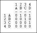
Suppose that we had a simple directed relation, represented as a matrix as in figure 6.9.
Figure 6.9. Linegraph example matrix
This is easier to see as a graph, as in figure 6.10.
Figure 6.10. Linegraph example graph
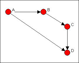
Now suppose that we are really interested in describing and thinking about the relations, and the relations among the relations -- rather than the actors, and the relations among them. That sounds odd, I realize. Let me put it a different way. We can think about the graph in Figure 6.5 as composed of four relations (A to B, B to C, C to D, and A to C). These relations are connected by having actors in common (e.g. the A to B and the B to C relations have the actor B in common). That is, we can think about relations as being "adjacent" when they share actors, just as we can think about actors being adjacent when they share relations.
Transform>Incidence is an algorithm that changes the way we look at a directed graph from "actors connected by relations" to "relations connected by actors." This is sometimes just a semantic trick. But, sometimes it's more than that -- our theory of the social structure may actually be one about which relations are connected, not which actors are connected. If we apply the Transform>Incidence algorithm to the data in figures 6.4 and 6.5, we get the result in figure 6.11.
Figure 6.11. Incidence matrix of graph 6.10
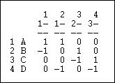
Each row is an actor. Each column is now a relation (the relations are numbered 1 through 4). A positive entry indicates that an actor is the source of a a directed relation. For example, actor A is the origin of the relation "1" that connects A to B, and is a source of the relation "2" that connects actor A to actor D. A negative entry indicates that an actor is the "sink" or recipient of a directed relation. For example, actor C is the recipient in relation "3" (which connects actor B to actor C), and the source of relation "4" (which connects actor C to actor D.
The "incidence" matrix here then shows how actors are connected to relationships. By examining the rows, we can characterize how much, and in what ways actors are embedded in relations. One actor may have few entries -- a near isolate; another may have many negative and few positive entries -- a "taker" rather than a "giver." By examining the columns, we get a description of which actors are connected, in which way, by each of the relations in the graph.
Focusing on the relations, instead of the actors
Turning an actor-by-actor adjacency matrix into an actor-by-relation incidence graph takes us part of the way toward focusing on relations rather than actors. We can go further.
Transform> Linegraph converts an actor-by-actor matrix (like figure 6.4) into a full relation-by-relation matrix. Figure 6.12 shows the results of applying it to the example data.
Figure 6.12. Linegraph matrix
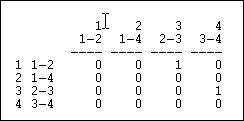
We again have a square matrix. This time, though, it describes which relations in the graph are "adjacent to" which other relations. Two relations are adjacent if they share an actor. For example, relation "1" (the tie between actors 1 and 2, or A and B) is adjacent to the relation "3" (the tie between actors 2 and 3, or B and C). Note that the "adjacency" here is directional -- relation 1 is a source of relation 3. We could also apply this approach to symmetric or simple graphs to describe which relations are simply adjacent in a un-directed way.
A quick glance at the linegraph matrix is suggestive. It is very sparse in this example -- most of the relations are not sources of other relations. The maximum degree of each entry is 1 -- no relation is the source of multiple relations. While there may be a key or central actor (A), it's not so clear that there is a single central relation.
To be entirely honest, most social network analysts do (much of the time) think about actors connected to actors by relations, rather than relations connecting actors, or relations connecting relations. But changing our point of view to put the relations first, and the actors second is, in many ways, a more distinctively "sociological" way of looking at networks. Transforming actor-by-actor data into relation-by-relation data can yield some interesting insights about social structures.
table of contentsIn this chapter we've covered a number of rather diverse but related topics. We've described some of the basic "nuts and bolts" tools for entering and transforming network data. The "bigger picture" is to think about network data (and any other, for that matter) as having "structure." Once you begin to see data in this way, you can begin to better imagine the creative possibilities: for example, treating actor-by-attribute data as actor-by-actor, or treating it as attribute-by-attribute. Different research problems may call for quite different ways of looking at, and transforming, the same data structures. We've hardly covered every possibility here, but we have looked at some of the most frequently used tricks.