5. Using matrices to represent social relations
Graphs are very useful ways of presenting information about social networks. However, when there are many actors and/or many kinds of relations, they can become so visually complicated that it is very difficult to see patterns. It is also possible to represent information about social networks in the form of matrices. Representing the information in this way also allows the application of mathematical and computer tools to summarize and find patterns. Social network analysts use matrices in a number of different ways. So, understanding a few basic things about matrices from mathematics is necessary. We'll go over just a few basics here that cover most of what you need to know to understand what social network analysts are doing. For those who want to know more, there are a number of good introductory books on matrix algebra for social scientists.
To start with, a matrix is nothing more than a rectangular arrangement of a set of elements (actually, it's a bit more complicated than that, but we will return to matrices of more than two dimensions in a little bit). Rectangles have sizes that are described by the number of rows of elements and columns of elements that they contain. A "3 by 6" matrix has three rows and six columns; an "I by j" matrix has I rows and j columns. A matrix that has only one row is called a "row vector." A matrix that has only one column is called a "column vector.
Figure 5.1 shows a two-by-four matrix. Figure 5.2 shows a four by two matrix. Just for the moment, ignore the contents of the cells (e.g. 1,1).
Figure 5.1. Example of a "two-by-four" matrix
| 1,1 | 1,2 | 1,3 | 1,4 |
| 2,1 | 2,2 | 2,3 | 2,4 |
Figure 5.2. Example of at "four-by-two" matrix
| 1,1 | 1,2 |
| 2,1 | 2,2 |
| 3,1 | 3,2 |
| 4,1 | 4,2 |
The elements (cells) of a matrix are identified by their "addresses." Element 1,1 is the entry in the first row and first column; element 13,2 is in the 13th row and is the second element of that row. The cell addresses have been entered as matrix elements in the two examples above.
Matrices are often represented as arrays of elements surrounded by vertical lines at their left and right, or square brackets at the left and right. In web pages it's easier to use "tables" to represent matrices. Matrices can be given names; these names are usually presented as capital bold-faced letters. Social scientists using matrices to represent social networks often dispense with the mathematical conventions, and simply show their data as an array of labeled rows and columns. The labels are not really part of the matrix, but are simply for clarity of presentation. The matrix in figure 5.3 for example, is a 4 by 4 matrix, with additional labels.
Figure 5.3. Four-by-four matrix with additional row and column labels
| A | B | C | D | |
| A |
--- |
1 |
0 |
0 |
| B |
1 |
--- |
1 |
0 |
| C |
1 |
1 |
--- |
1 |
| D |
0 |
0 |
1 |
--- |
The matrices used in social network analysis are frequently "square." That is, they contain the same number of rows and columns. But "rectangular" matrices are also used, as are row and column vectors. The same conventions apply to all these variations.
Occasionally, social network analysts will use a "3-dimensional" matrix. A three dimensional matrix has rows, columns, and "levels" or "slices." Each "slice" has the same rows and columns as each other slice. UCINET thinks about these more complicated 3-dimensional arrays of data as a collection of two-dimensional matrices.
The most common form of matrix in social network analysis is a very simple square matrix with as many rows and columns as there are actors in our data set. The "elements" or scores in the cells of the matrix record information about the ties between each pair of actors.
The simplest and most common matrix is binary. That is, if a tie is present, a one is entered in a cell; if there is no tie, a zero is entered. This kind of a matrix is the starting point for almost all network analysis, and is called an "adjacency matrix" because it represents who is next to, or adjacent to whom in the "social space" mapped by the relations that we have measured.
An adjacency matrix may be "symmetric" or "asymmetric." Social distance can be either symmetric or asymmetric. If Bob and Carol are "friends" they share a "bonded tie" and the entry in the Xi,j cell will be the same as the entry in the Xj,i cell.
But social distance can be a funny (non-Euclidean) thing. Bob may feel close to Carol, but Carol may not feel the same way about Bob. In this case, the element showing Bob's relationship to Carol would be scored "1," while the element showing Carol's relation to Bob would be scored "0." That is, in an "asymmetric" matrix, Xi,j is not necessarily equal to Xj,i.
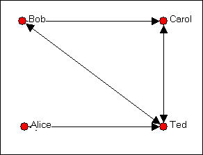
By convention, in a directed (i.e. asymmetric) matrix, the sender of a tie is the row and the target of the tie is the column. Let's look at a simple example. The directed graph of friendship choices among Bob, Carol, Ted, and Alice is shown in figure 5.4.
Figure 5.4 Bob, Carol, Ted, and Alice
We can since the ties are measured at the nominal level (that is, the data are binary choice data), we can represent the same information in a matrix that looks like:
Figure 5.5. Asymmetric adjacency matrix of the graph shown in figure 5.4.
| Bob | Carol | Ted | Alice | |
| Bob |
--- |
1 |
1 |
0 |
| Carol |
0 |
--- |
1 |
0 |
| Ted |
1 |
1 |
--- |
1 |
| Alice |
0 |
0 |
1 |
--- |
Remember that the rows represent the source of directed ties, and the columns the targets; Bob chooses Carol here, but Carol does not choose Bob. This is an example of an "asymmetric" matrix that represents directed ties (ties that go from a source to a receiver). That is, the element i,j does not necessarily equal the element j,i. If the ties that we were representing in our matrix were "bonded-ties" (for example, ties representing the relation "is a business partner of" or "co-occurrence or co-presence," (e.g. where ties represent a relation like: "serves on the same board of directors as") the matrix would necessarily be symmetric; that is element i,j would be equal to element j,i.
Binary choice data are usually represented with zeros and ones, indicating the presence or absence of each logically possible relationship between pairs of actors.
Signed graphs are represented in matrix form (usually) with -1, 0, and +1 to indicate negative relations, no or neutral relations, and positive relations. "Signed" graphs are actually a specialized version of an ordinal relation.
When ties are measured at the ordinal or interval level, the numeric magnitude of the measured tie is entered as the element of the matrix. As we discussed earlier, other forms of data are possible (multi-category nominal, ordinal with more than three ranks, full-rank order nominal). These other forms, however, are rarely used in sociological studies, and we won't give them very much attention.
In representing social network data as matrices, the question always arises: what do I do with the elements of the matrix where i = j? That is, for example, does Bob regard himself as a close friend of Bob? This part of the matrix is called the main diagonal. Sometimes the value of the main diagonal is meaningless, and it is ignored (and left blank or filled with zeros or ones). Sometimes, however, the main diagonal can be very important, and can take on meaningful values. This is particularly true when the rows and columns of our matrix are "super-nodes" or "blocks." More on that in a minute.
It is often convenient to refer to certain parts of a matrix using shorthand terminology. If I take all of the elements of a row (e.g. who Bob chose as friends: ---,1,1,0) I am examining the "row vector" for Bob. If I look only at who chose Bob as a friend (the first column, or ---,0,1,0), I am examining the "column vector" for Bob. It is sometimes useful to perform certain operations on row or column vectors. For example, if I summed the elements of the column vectors in this example, I would be measuring how "popular" each node was (in terms of how often they were the target of a directed friendship tie). So a "vector" can be an entire matrix (1 x ... or ...x 1), or a part of a larger matrix.
return to the table of contents of this page
It is also helpful, sometimes, to rearrange the rows and columns of a matrix so that we can see patterns more clearly. Shifting rows and columns (if you want to rearrange the rows, you must rearrange the columns in the same way, or the matrix won't make sense for most operations) is called "permutation" of the matrix.
Our original data look like figure 5.6:
Figure 5.6. Asymmetric adjacency matrix
| Bob | Carol | Ted | Alice | |
| Bob | --- | 1 | 1 | 0 |
| Carol | 0 | --- | 1 | 0 |
| Ted | 1 | 1 | --- | 1 |
| Alice | 0 | 0 | 1 | --- |
Let's rearrange (permute) this so that the two males and the two females are adjacent in the matrix. Matrix permutation (Data>Permute) simply means to change the order of the rows and columns. Since the matrix is symmetric, if I change the position of a row, I must also change the position of the corresponding column. The result is shown in figure 5.7.
Figure 5.7. Permuted matrix
| Bob | Ted | Carol | Alice | |
| Bob | --- | 1 | 1 | 0 |
| Ted | 1 | --- | 1 | 1 |
| Carol | 0 | 1 | --- | 0 |
| Alice | 0 | 1 | 0 | --- |
None of the elements have had their values changed by this operation or rearranging the rows and columns, we have just shifted things around. We've also highlighted some sections of the matrix. Each colored section is referred to as a block. Blocks are formed by passing dividing lines through the matrix (e.g. between Ted and Carol) rows and columns. Passing these dividing lines through the matrix is called partitioning the matrix. Here we have partitioned by the actor by their sex. Partitioning is also sometimes called "blocking the matrix," because partitioning produces blocks.
This kind of grouping of cells is often done in network analysis to understand how some sets of actors are "embedded" in social roles or in larger entities. Here, for example, we can see that all occupants of the social role "male" choose each other as friends; no females choose each other as friends, and that males are more likely to choose females (3 out of 4 possibilities are selected) than females are to choose males (only 2 out of 4 possible choices). We have grouped the males together to create a "partition" or "super-node" or "social role" or "block." We often partition social network matrices in this way to identify and test ideas about how actors are "embedded" in social roles or other "contexts."
We might wish to dispense with the individual nodes altogether, and examine only the positions or roles. If we calculate the proportion of all ties within a block that are present, we can create a block density matrix. In doing this, we have ignored self-ties in figure 5.8.
Figure 5.8. Block density matrix
| Male | Female | |
| Male | 1.00 | 0.75 |
| Female | 0.50 | 0.00 |
We may wish to summarize the information still further by using block image or image matrix. If the density in a block is greater than some amount (we often use the average density for the whole matrix as a cut-off score, in the current example the density is .58), we enter a "1" in a cell of the blocked matrix, and a "0" otherwise. This kind of simplification is called the "image" of the blocked matrix, as in figure 5.9.
Figure 5.9. Image matrix of sex blocked data, using overall mean density as the cut-off
| Male | Female | |
| Male |
1 |
1 |
| Female |
0 |
0 |
Images of blocked matrices are powerful tools for simplifying the presentation of complex patterns of data. Like any simplifying procedure, good judgment must be used in deciding how to block and what cut-offs to use to create images -- or we may lose important information.
UCINET includes tools that make permuting and blocking matrices rather easy.
Transform>Block allows you to select a matrix to be blocked, a row and/or column partition, and a method for calculating the entries in the resulting blocks.
To use this command, you need to first create separate files that describe the row partition and the column partition. These files are simply vectors (either one row, or one column) that identify which actors are to fall into which partition. For example, if actors 1, 2, and 5 were to form group A, and actors 3 and 4 were to form group B, my column partition data set would read: 1 1 2 2 1. These partitions or blockings are simply regular UCINET data files with one row or one column.
The command asks for a method of summarizing the information within each block. You may take the average of the values in the block (if the data are binary, taking the average is the same thing as calculating the density), sum the values in the block, select the highest value or the lowest value, or select a measure of the amount of variation among the scores in the block -- either the sums of squares or the standard deviation.
The command outputs two new matrices. The "PreImage" data set contains the original scores, but permuted; the "Reduced image dataset" contains a new block matrix containing the block densities.
Transform>Collapse allows you to combine rows and/or columns by specifying (detailed instructions are given on the command window) which elements are to be combined, and how. We might select, for example, to combine columns 1, 2, and 5, and rows 1, 2, and 5 by taking the average of the values (we could also select the maximum, minimum, or sum). The command creates a new matrix that has collapsed the desired rows or columns using the summary operation you selected.
The data menu also gives you some tools for this kind of work:
Data>Permute allows you to re-arrange the rows and/or columns and/or matrices (if your data set contains multiple matrices representing multiple relations, like the Knoke bureaucracies "information" and "money" relations). You simply specify the new order with a list. If I wanted to group rows 1, 2, and 5 to be new rows 1, 2, and 3; and rows 3 and 4 to be new rows 4 and 5, I would enter 1 2 4 5 3.
Data>Sort re-arranges the rows, columns, or both of the matrix according to a criterion you select. If you data are valued (i.e. represent tie strength) you might want to sort the rows and columns in ascending or descending order (this could make sense for binary data, too). If you want a more complicated sort (say "all the 3's first, then all the 1's, then all the 2's) you can use an external UCINET data file to specify this as a vector (i.e. the data set would just be: 3 1 2).
Data>Transpose re-arranges the data in a way that is very commonly used in matrix algebra -- by taking the "transpose." A transpose is, very simply, switching the rows and columns of a matrix for one another.
Representing the ties among actors as matrices can help us to see patterns by performing simple manipulations like summing row vectors or partitioning the matrix into blocks. Social network analysts use a number of other mathematical operations that can be performed on matrices for a variety of purposes (matrix addition and subtraction, transposes, inverses, matrix multiplication, and some other more exotic stuff like determinants and eigenvalues). Without trying to teach you matrix algebra, it is useful to know at least a little bit about some of these mathematical operations, and what they are used for in social network analysis.
UCINET has built-in functions for doing most matrix algebra functions. Look under the Tools>Matrix Algebra menu. If you do know some matrix algebra, you will find that this tool lets you do almost anything to matrix data that you may desire. But, you do need to know what you are doing. The help screen for this command shows how to identify the matrix or matrices that are to be manipulated, and the algorithms that can be applied.
This simply means to exchange the rows and columns so that i becomes j, and vice versa. If we take the transpose of a directed adjacency matrix and examine its row vectors (you should know all this jargon by now!), we are looking at the sources of ties directed at an actor. The degree of similarity between an adjacency matrix and the transpose of that matrix is one way of summarizing the degree of symmetry in the pattern of relations among actors. That is, the correlation between an adjacency matrix and the transpose of that matrix is a measure of the degree of reciprocity of ties (think about that assertion a bit). Reciprocity of ties can be a very important property of a social structure because it relates to both the balance and to the degree and form of hierarchy in a network. This command is also available as Data>Transpose.
Taking the inverse of a matrix
This is a mathematical operation that finds a matrix which, when multiplied by the original matrix, yields a new matrix with ones in the main diagonal and zeros elsewhere (which is called an identity matrix). Without going any further into this, you can think of the inverse of a matrix as being sort of the "opposite of" the original matrix. Matrix inverses are used mostly in calculating other things in social network analysis. They are sometimes interesting to study in themselves, however. It is sort of like looking at black lettering on white paper versus white lettering on black paper: sometimes you see different things. Inverses are calculated with Tools>Matrix Algebra.
Matrix addition and matrix subtraction
These are the easiest of matrix mathematical operations. One simply adds together or subtracts each corresponding i,j element of the two (or more) matrices. Of course, the matrices that this is being done to have to have the same numbers of I and j elements (this is called "conformable" to addition and subtraction) - and, the values of i and j have to be in the same order in each matrix.
Matrix addition and subtraction are most often used in network analysis when we are trying to simplify or reduce the complexity of multiplex (multiple relations recorded as separate matrices or slices) data to simpler forms. If I had a symmetric matrix that represented the tie "exchanges money" and another that represented the relation "exchanges goods" I could add the two matrices to indicate the intensity of the exchange relationship. Pairs with a score of zero would have no relationship, those with a "1" would be involved in either barter or commodity exchange, and those with a "2" would have both barter and commodity exchange relations. If I subtracted the "goods" exchange matrix from the "money exchange" matrix, a score of -1 would indicate pairs with a barter relationship; a score of zero would indicate either no relationship or a barter and commodity tie; a score of +1 would indicate pairs with only a commodified exchange relationship. For different research questions, either or both approaches might be useful. Tools>Matrix Algebra are one way of doing these sorts of data transformations.
Matrix multiplication and Boolean matrix multiplication
Matrix multiplication is a somewhat unusual operation, but can be very useful for the network analyst. You will have to be a bit patient here. First we need to show you how to do matrix multiplication and a few important results (like what happens when you multiply an adjacency matrix times itself, or raise it to a power). Then, we will try to explain why this is useful.
To multiply two matrices, they must be "conformable" to multiplication. This means that the number of rows in the first matrix must equal the number of columns in the second. Usually network analysis uses adjacency matrices, which are square, and hence, conformable for multiplication. Multiplying a matrix by itself (i.e. raising it to a power) and multiplying a square matrix by its transpose are obviously "conformable." Unlike regular multiplication of individual numbers X*Y is not the same thing as Y*X in matrix multiplication -- the order matters!
To multiply two matrices, begin in the upper left hand corner of the first matrix, and multiply every cell in the first row of the first matrix by the values in each cell of the first column of the second matrix, and sum the results. Proceed through each cell in each row in the first matrix, multiplying by the column in the second. To perform a Boolean matrix multiplication, proceed in the same fashion, but enter a zero in the cell if the multiplication product is zero, and one if it is not zero. An example helps. Suppose we wanted to multiply the two matrices in figure 5.10.
Figure 5.10. Two matrices to be multiplied.
| 0 | 1 |
| 2 | 3 |
| 4 | 5 |
times
| 6 | 7 | 8 |
| 9 | 10 | 11 |
The result is shown in figure 5.11.
Figure 5.11. Result of matrix multiplication.
| (0*6)+(1*9) | (0*7)+(1*10) | (0*8)+(1*11) |
| (2*6)+(3*9) | (2*7)+(3*10) | (2*8)+(3*11) |
| (4*6)+(5*9) | (4*7)+(5*10) | (4*8)+(5*11) |
The mathematical operation in itself doesn't interest us here (any number of programs can perform matrix multiplication). But, the operation is useful when applied to an adjacency matrix. Consider our four friends again, in figure 5.12.
Figure 5.12. Directed graph of friendship relations among Bob, Carol, Ted, and Alice
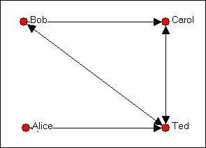
The adjacency matrix for the four actors B, C, T, and A (in that order) is shown as figure 5.13.
Figure 5.13. Adjacency matrix for graph in figure 5.12.
|
--- |
1 |
1 |
0 |
|
0 |
--- |
1 |
0 |
|
1 |
1 |
--- |
1 |
|
0 |
0 |
1 |
--- |
Another way of thinking about this matrix is to notice that it tells us whether there is a path from each actor to each actor. A one represents the presence of a path, a zero represents the lack of a path. The adjacency matrix is exactly what its name suggests -- it tells us which actors are adjacent, or have a direct path from one to the other.
Now suppose that we multiply this adjacency matrix times itself (i.e. raise the matrix to the 2nd power, or square it). We will treat "self-ties" as zeros, which, effectively, ignores them. The calculation of the matrix squared is shown as figure 5.14.
Figure 5.14. Squaring matrix 5.13.
| (0*0)+(1*0)+(1*1)+(0*0) | (0*1)+(1*0)+(1*1)+(0*0) | (0*1)+(1*1)+(1*0)+(0*1) | (0*0)+(1*0)+(1*1)+(0*0) |
| (0*0)+(0*0)+(1*1)+(0*0) | (0*1)+(0*0)+(1*1)+(0*0) | (0*1)+(0*1)+(1*0)+(0*1) | (0*0)+(0*0)+(1*1)+(0*0) |
| (1*0)+(1*0)+(0*1)+(1*0) | (1*1)+(1*0)+(0*1)+(1*0) | (1*1)+(1*1)+(0*0)+(1*1) | (1*0)+(1*0)+(0*1)+(1*0) |
| (0*0)+(0*0)+(1*1)+(0*0) | (0*1)+(0*0)+(1*1)+(0*0) | (0*1)+(0*1)+(1*0)+(0*1) | (0*0)+(0*0)+(1*1)+(0*0) |
|
1 |
1 |
1 |
1 |
|
1 |
1 |
0 |
1 |
|
0 |
1 |
3 |
0 |
|
1 |
1 |
0 |
1 |
So, the adjacency matrix tells us how many paths of length one are there from each actor to each other actor. The adjacency matrix squared tells us how many pathways of length two are there from each actor to each other actor. It is true (but we won't show it to you) that the adjacency matrix cubed counts the number of pathways of length three from each actor to each other actor. And so on...
If we calculated the Boolean product, rather than the simple matrix product, the adjacency matrix squared would
tell us whether there was a path of length two between two actors (not how many such paths there were). If we took
the Boolean squared matrix and multiplied it by the adjacency matrix using Boolean multiplication, the result would
tell us which actors were connected by one or more pathways of length three. And so on...
Now, finally: why should you care?
Some of the most fundamental properties of a social network have to do with how connected the actors are to one another. Networks that have few or weak connections, or where some actors are connected only by pathways of great length may display low solidarity, a tendency to fall apart, slow response to stimuli, and the like. Networks that have more and stronger connections with shorter paths among actors may be more robust and more able to respond quickly and effectively. Measuring the number and lengths of pathways among the actors in a network allow us to index these important tendencies of whole networks.
Individual actor's positions in networks are also usefully described by the numbers and lengths of pathways that they have to other actors. Actors who have many pathways to other actors may be more influential with regard to them. Actors who have short pathways to more other actors may me more influential or central figures. So, the number and lengths of pathways in a network are very important to understanding both individual's constraints and opportunities, and for understanding the behavior and potentials of the network as a whole.
There are many measures of individual position and overall network structure that are based on whether there are pathways of given lengths between actors, the length of the shortest pathway between two actors, and the numbers of pathways between actors. Indeed, most of the basic measures of networks, measures of centrality and power, and measures of network groupings and substructures are based on looking at the numbers and lengths of pathways among actors.
For most analyses, you won't have to manipulate matrices -- UCINET and other programs have already built algorithms that have the compute do these operations. Most of the computational work in network analysis is done with matrix mathematics though, so in order to understand what is going on, it's useful to understand the basics.
Matrices are collections of elements into rows and columns. They are often used in network analysis to represent the adjacency of each actor to each other actor in a network. An adjacency matrix is a square actor-by-actor (i=j) matrix where the presence of pair wise ties are recorded as elements. The main diagonal, or "self-tie" of an adjacency matrix is often ignored in network analysis.
Sociograms, or graphs of networks can be represented in matrix form, and mathematical operations can then be performed to summarize the information in the graph. Vector operations, blocking and partitioning, and matrix mathematics (inverses, transposes, addition, subtraction, multiplication and Boolean multiplication), are mathematical operations that are sometimes helpful to let us see certain things about the patterns of ties in social networks.
Social network data are often multiplex (i.e. there are multiple kinds of ties among the actors). Such data are represented as a series of matrices of the same dimension with the actors in the same position in each matrix. Many of the same tools that we can use for working with a single matrix (matrix addition and correlation, blocking, etc.) Are helpful for trying to summarize and see the patterns in multiplex data.
Once a pattern of social relations or ties among a set of actors has been represented in a formal way (graphs or matrices), we can define some important ideas about social structure in quite precise ways using mathematics for the definitions. In the remainder of the book, we will look at how social network analysts have formally translated some of the core concepts that social scientists use to describe social structures.
1. A matrix is "3 by 2." How many columns does it have? How many rows?
2. Adjacency matrices are "square" matrices. Why?
3. There is a "1" in cell 3,2 of an adjacency matrix representing a sociogram. What does this tell us?
4. What does it mean to "permute" a matrix, and to "block" it?
Application questions
1. Think of the readings from the first part of the course. Did any studies present matrices? If they did, what kinds of matrices were they (that is, what is the technical description of the kind of graph or matrix). Pick one article, and show what the data would look like, if represented in matrix form.
2. Think of some small group of which you are a member (maybe a club, or a set of friends, or people living in the same apartment complex, etc.). What kinds of relations among them might tell us something about the social structures in this population? Try preparing a matrix to represent one of the kinds of relations you chose. Can you extend this matrix to also describe a second kind of relation? (e.g. one might start with "who likes whom?" and add "who spends a lot of time with whom?").
3. Using the matrices you created in the previous question, does it make sense to leave the diagonal "blank," or not, in your case? Try permuting your matrix, and blocking it.
4. Can you make an adjacency matrix to represent the "star" network? what about the "line" and "circle." Look at the ones and zeros in these matrices -- sometimes we can recognize the presence of certain kinds of social relations by these "digital" representations. What does a strict hierarchy look like? What does a population that is segregated into two groups look like?